5. Geospatial python

Because of the wide array (pun intended) of open source data science modules that are accessible with python, it has emerged as a flagship language for processing, analyzing, and visualizing geospatial data. There are several key geospatial packages available in python:

• Geopandas - processing vector data (e.g. shapfiles, .GeoJSON, .KML, see here for a full list of geospatial vector filetypes)

• Rasterio - processing raster data (e.g. satellite imagery in .tif or .tiff format)

• Xarray - multidimensional array analysis (e.g. time series gridded or satellite datasets in .nc or .hdf format)

• GDAL - the key library (originally written in C and C++) that underscores most of the raster and vector processing operations in the above libraries, as well as GUI-based GIS software (ArcMap, QGIS, Google Earth/Maps, etc)

We will begin with (1) an (abridged) overview of map projections and coordinate systems, and (2) a brief discussion of the two fundamental types of geospatial data to motivate the topic.

Coordinate Systems and Projections

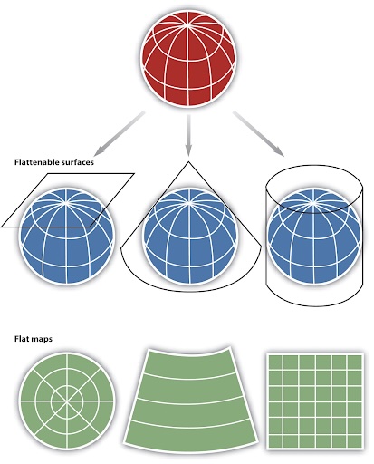
A coordinate system is a framework used to determine position on the surface of the earth. Coordinate Systems are practical solutions to the challenge of depicting a 3D object (the earth) on a 2D surface (a screen).

Example of a coordinate system for a 2-D plane is the Cartesian Coordinate System (i.e. X and Y)

You’ve probably seen the Geographic Coordinate System (GCS), the three-dimensional coordinate system commonly used to define locations on the earth’s surface.

• The unit of measure in the GCS is degrees,

• locations are defined by latitude and longitude

A Map Projection is how we transform geographic data from a three-dimensional, spherical coordinate system to a two-dimensional planar system. Map projections introduce distortions in distance, direction, and area. They are useful to convert data with units of degrees (in a GCS) into more practical length units such as meters or feet. There are several types of projected coordinate systems and projection types that can be used, the most common being:

• Planar

• Conical

• Cylindrical

Vector and Raster data

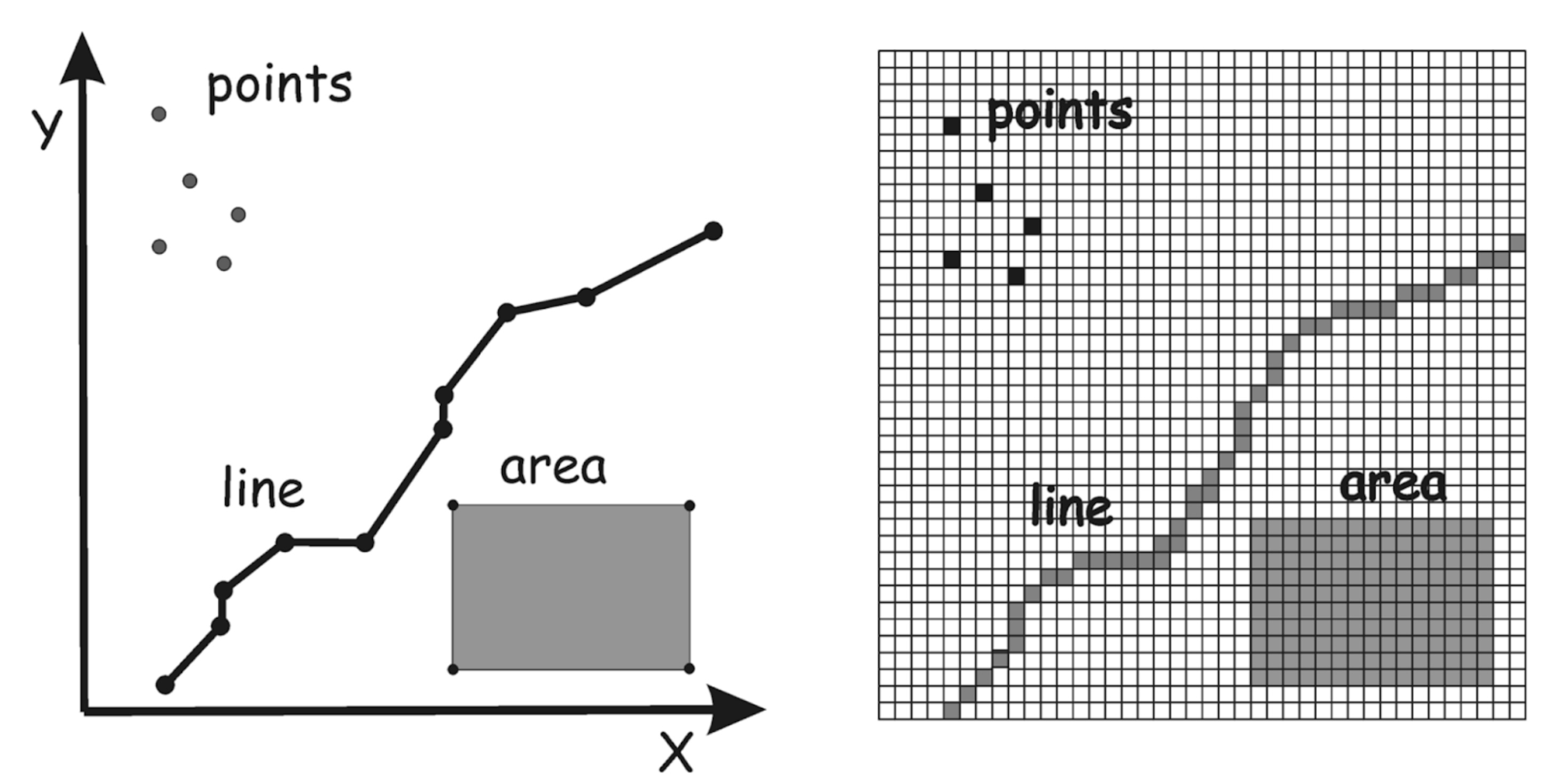
Geospatial data can be broadly categorized as either Vector or Raster:

Vector

• Vector data consit of points, lines, and polygons

• Stored as tabular data files with geographic metadata

• Lines are made up of points, have a starting and ending point

• Polygons are made up of points, and the starting point = the ending point.

• Can have a topology, or an organizational scheme to e.g. dictate the order or direction of data

Raster

• Raster data consist of grids of numbers - ‘Raster’ means ‘screen’ in Latin

• Can contain multiple channels / bands - a true color image has Red, Green, Blue channels

• The Spatial Resolution of a raster image refers to the size of a pixel (e.g. 1mm, 1cm, or 1m)

• Satellite / drone / camera data is natively raster

The below image shows vector data on the left, and raster data on the right:

Now that we have some foundational Geospatial knowledge under our belt, let’s cover some of the python tools that we can use to process, analyze, and visualize geospatial data:

Geopandas

Remember pandas from last module? Enter geopandas - a natural geospatial extension to store tabular vector data (think points, lines, and polygons) and simplify operations by keeping with pandas-like syntax.

Let’s load the same stations.csv file and convert it from a pandas.DataFrame to a geopandas.GeoDataFrame:

import pandas as pd

url = "https://raw.githubusercontent.com/py4wrds/py4wrds/refs/heads/module-4/data/gwl/stations.csv"
df = pd.read_csv(url)

df.head()

	STN_ID	SITE_CODE	SWN	WELL_NAME	LATITUDE	LONGITUDE	WLM_METHOD	WLM_ACC	BASIN_CODE	BASIN_NAME	COUNTY_NAME	WELL_DEPTH	WELL_USE	WELL_TYPE	WCR_NO	ZIP_CODE
0	51445	320000N1140000W001	NaN	Bay Ridge	35.5604	-121.755	USGS quad	Unknown	NaN	NaN	Monterey	NaN	Residential	Part of a nested/multi-completion well	NaN	92154
1	25067	325450N1171061W001	19S02W05K003S	NaN	32.5450	-117.106	Unknown	Unknown	9-033	Coastal Plain Of San Diego	San Diego	NaN	Unknown	Unknown	NaN	92154
2	25068	325450N1171061W002	19S02W05K004S	NaN	32.5450	-117.106	Unknown	Unknown	9-033	Coastal Plain Of San Diego	San Diego	NaN	Unknown	Unknown	NaN	92154
3	39833	325450N1171061W003	19S02W05K005S	NaN	32.5450	-117.106	Unknown	Unknown	9-033	Coastal Plain Of San Diego	San Diego	NaN	Unknown	Unknown	NaN	92154
4	25069	325450N1171061W004	19S02W05K006S	NaN	32.5450	-117.106	Unknown	Unknown	9-033	Coastal Plain Of San Diego	San Diego	NaN	Unknown	Unknown	NaN	92154

# Create a GeoDataFrame from the DataFrame

import geopandas as gpd

gdf_stns = gpd.GeoDataFrame(
    df,
    geometry=gpd.points_from_xy(df["LONGITUDE"], df["LATITUDE"]),
    crs="EPSG:4326",  # Set the coordinate reference system (CRS) - more on this later
)

GeoDataFrame objects are a subclass of pandas.DataFrame, so you can use all of the same methods. In fact, a GeoDataFrame is just a pandas.DataFrame with a single extra column (geometry) and some extra features that make use of that column.

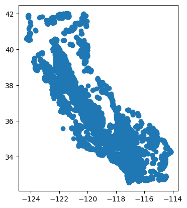
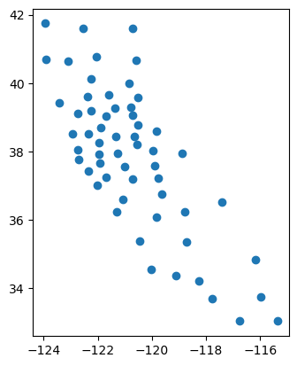
plot() is a special geopandas method that will plot the geometry / latlon of the df:

# Plot our results:
gdf_stns.plot()

<Axes: >

When printed, the tabular data is identical, and all pandas-like syntax can be used to sort and filter data:

# Get unique county names
print(gdf_stns["COUNTY_NAME"].unique())
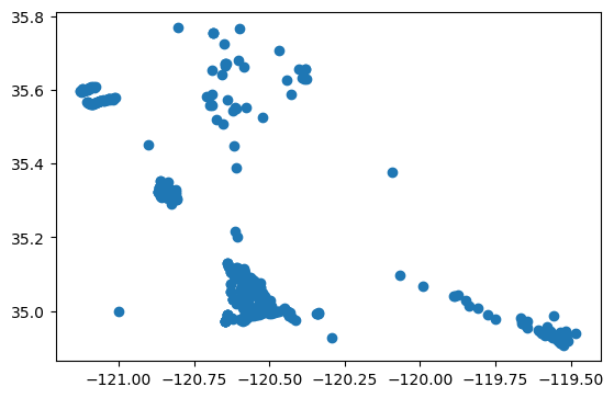
# Plotting all stations in SLO county only
gdf_stns[gdf_stns["COUNTY_NAME"] == "San Luis Obispo"].plot()

['Monterey' 'San Diego' 'Imperial' 'Riverside' 'Orange' 'Kern'
 'Los Angeles' 'San Bernardino' 'Ventura' 'Santa Barbara' 'Alameda'
 'San Luis Obispo' 'Amador' 'Alpine' 'Tulare' 'Inyo' 'Fresno' 'Kings'
 'Merced' 'San Benito' 'San Joaquin' 'Glenn' 'Madera' 'Santa Cruz'
 'Santa Clara' 'Plumas' 'Stanislaus' 'San Mateo' 'Mono' 'Mariposa'
 'San Francisco' 'Contra Costa' 'Tuolumne' 'Marin' 'Calaveras' 'Sonoma'
 'Sacramento' 'Sutter' 'Solano' 'Napa' 'Placer' 'Yolo' 'Lake' 'Colusa'
 'El Dorado' 'Mendocino' 'Yuba' 'Butte' 'Nevada' 'Sierra' 'Lassen'
 'Tehama' 'Shasta' 'Humboldt' 'Modoc' 'Siskiyou' 'Del Norte' 'Klamath, OR']

<Axes: >

Reading and writing vector files

Geopandas excels at making it easy to read and write vector files of several formats, which facilitates conversions and interoperability.

Simply import geopandas as gpd and then read any common vector file format with the gpd.read_file('filename') function, which works for common formats such as .shp (and supporting .dbf and .shx files), kml, kmz, geojson, etc..

# Read a geojson file
url = "https://raw.githubusercontent.com/scottpham/california-counties/refs/heads/master/caCountiesTopo.json"
gdf_counties = gpd.read_file(url)
gdf_counties.head()

	id	name	fullName	areaLand	geometry
0	06091	Sierra	Sierra County	2468686345	POLYGON ((-120.14666 39.70738, -120.13527 39.7...
1	06067	Sacramento	Sacramento County	2499176690	POLYGON ((-121.14147 38.7118, -121.14043 38.71...
2	06083	Santa Barbara	Santa Barbara County	7083926262	MULTIPOLYGON (((-119.46758 34.06296, -119.4862...
3	06009	Calaveras	Calaveras County	2641819811	POLYGON ((-120.07212 38.50985, -120.07212 38.5...
4	06111	Ventura	Ventura County	4773381212	MULTIPOLYGON (((-119.63631 33.27314, -119.6363...

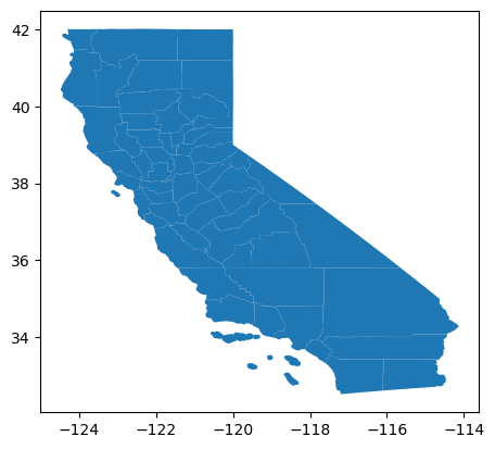
gdf_counties.plot()

<Axes: >

To write files, simply use the syntax: gdf.to_file("path/to/out_file.geojson") syntax. We recommend storing files as .geojson due to readability and simplicity to store and retrieve.

gdf_counties.to_file("ca_counties.geojson")

/Users/andrew/opt/miniconda3/envs/py4wrds2/lib/python3.13/site-packages/pyogrio/geopandas.py:662: UserWarning: 'crs' was not provided.  The output dataset will not have projection information defined and may not be usable in other systems.
  write(

We received a warning that our CRS was not defined. We can eliminate this warning by defining the geographic WGS 84 coordinate reference system (CRS) through its EPSG code using gdf.set_crs('epsg:4236').

Similar to other DataFrame and pandas operations, we must specify the inplace = True argument:

gdf_counties.set_crs("epsg:4326", inplace=True)
gdf_counties.to_file("ca_counties.geojson")

# verify that file was written in our current directory:
import os

[x for x in os.listdir(os.getcwd()) if "geojson" in x]

['ca_counties.geojson']

We can inspect the coordinate reference system by using the gdf.crs syntax:

# Geographic CRS example:
gdf_stns.crs

<Geographic 2D CRS: EPSG:4326>
Name: WGS 84
Axis Info [ellipsoidal]:
- Lat[north]: Geodetic latitude (degree)
- Lon[east]: Geodetic longitude (degree)
Area of Use:
- name: World.
- bounds: (-180.0, -90.0, 180.0, 90.0)
Datum: World Geodetic System 1984 ensemble
- Ellipsoid: WGS 84
- Prime Meridian: Greenwich

Reprojections

Often, we’ll want to change the coordinate system of some data. This can be achieved through reprojection.

UTM zones:

Universal Transverse Mercator (UTM) is often an appropriate coordinate system for measuring distances, areas, etc

• Units in meters, expressed in Easting / Northing

UTM coordinate systems

Let’s reproject the geodataframe into a projected CRS for California - UTM Zone 10 N, which is epsg:32611:

gdf_rpj = gdf_stns.to_crs("epsg:32611")
gdf_rpj.crs

<Projected CRS: EPSG:32611>
Name: WGS 84 / UTM zone 11N
Axis Info [cartesian]:
- E[east]: Easting (metre)
- N[north]: Northing (metre)
Area of Use:
- name: Between 120°W and 114°W, northern hemisphere between equator and 84°N, onshore and offshore. Canada - Alberta; British Columbia (BC); Northwest Territories (NWT); Nunavut. Mexico. United States (USA).
- bounds: (-120.0, 0.0, -114.0, 84.0)
Coordinate Operation:
- name: UTM zone 11N
- method: Transverse Mercator
Datum: World Geodetic System 1984 ensemble
- Ellipsoid: WGS 84
- Prime Meridian: Greenwich

the estimate_utm_crs() function may be convenient for going between geographic and projected CRS:

gdf_stns.estimate_utm_crs()

<Projected CRS: EPSG:32611>
Name: WGS 84 / UTM zone 11N
Axis Info [cartesian]:
- E[east]: Easting (metre)
- N[north]: Northing (metre)
Area of Use:
- name: Between 120°W and 114°W, northern hemisphere between equator and 84°N, onshore and offshore. Canada - Alberta; British Columbia (BC); Northwest Territories (NWT); Nunavut. Mexico. United States (USA).
- bounds: (-120.0, 0.0, -114.0, 84.0)
Coordinate Operation:
- name: UTM zone 11N
- method: Transverse Mercator
Datum: World Geodetic System 1984 ensemble
- Ellipsoid: WGS 84
- Prime Meridian: Greenwich

Geometric Operations

We can easily calculate geometry properties such as area, centroids, bounds, and distances using geopandas.

Recall that one of our datasets consists of points (gdf_stns), and the other consists of polygons (gdf_counties)

Calculating Areas

# Calculate area for each polygon in a UTM CRS
# Note - the units depend on the coordinate system,
# Be sure to reproject appropriately and perform conversions

gdf_rpj["area_sqkm"] = gdf_rpj.area * 1e-6  # Sq m to sq km

gdf_rpj.head()

	STN_ID	SITE_CODE	SWN	WELL_NAME	LATITUDE	LONGITUDE	WLM_METHOD	WLM_ACC	BASIN_CODE	BASIN_NAME	COUNTY_NAME	WELL_DEPTH	WELL_USE	WELL_TYPE	WCR_NO	ZIP_CODE	geometry	area_sqkm
0	51445	320000N1140000W001	NaN	Bay Ridge	35.5604	-121.755	USGS quad	Unknown	NaN	NaN	Monterey	NaN	Residential	Part of a nested/multi-completion well	NaN	92154	POINT (68916.162 3945609.103)	0.0
1	25067	325450N1171061W001	19S02W05K003S	NaN	32.5450	-117.106	Unknown	Unknown	9-033	Coastal Plain Of San Diego	San Diego	NaN	Unknown	Unknown	NaN	92154	POINT (490047.407 3600852.39)	0.0
2	25068	325450N1171061W002	19S02W05K004S	NaN	32.5450	-117.106	Unknown	Unknown	9-033	Coastal Plain Of San Diego	San Diego	NaN	Unknown	Unknown	NaN	92154	POINT (490047.407 3600852.39)	0.0
3	39833	325450N1171061W003	19S02W05K005S	NaN	32.5450	-117.106	Unknown	Unknown	9-033	Coastal Plain Of San Diego	San Diego	NaN	Unknown	Unknown	NaN	92154	POINT (490047.407 3600852.39)	0.0
4	25069	325450N1171061W004	19S02W05K006S	NaN	32.5450	-117.106	Unknown	Unknown	9-033	Coastal Plain Of San Diego	San Diego	NaN	Unknown	Unknown	NaN	92154	POINT (490047.407 3600852.39)	0.0

Centroids

The centroid is the geographic center point of a polygon (i.e. the mean of all the points that make up its surface)

Calculating centroids can be done with the gdf.centroid function:

print(gdf_counties.centroid.head())
gdf_counties.centroid.plot()

0      POINT (-120.5159 39.5804)
1    POINT (-121.34431 38.44933)
2    POINT (-120.03075 34.53832)
3    POINT (-120.55404 38.20466)
4    POINT (-119.12598 34.35742)
dtype: geometry

/var/folders/df/w347rlh96tx42h1kl69_4r8w0000gn/T/ipykernel_73601/3389763898.py:1: UserWarning: Geometry is in a geographic CRS. Results from 'centroid' are likely incorrect. Use 'GeoSeries.to_crs()' to re-project geometries to a projected CRS before this operation.

  print(gdf_counties.centroid.head())
/var/folders/df/w347rlh96tx42h1kl69_4r8w0000gn/T/ipykernel_73601/3389763898.py:2: UserWarning: Geometry is in a geographic CRS. Results from 'centroid' are likely incorrect. Use 'GeoSeries.to_crs()' to re-project geometries to a projected CRS before this operation.

  gdf_counties.centroid.plot()

<Axes: >

the alpha keyword here gives a transparency to the plotted points with 0 being fully transparent and 1 being fully opaque

Boundaries

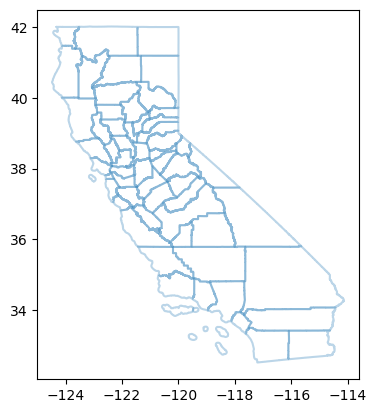
Similarly, boundaries can be obtained with the gdf.boundary function:

# Get the boundary of each polygon
print(gdf_counties.boundary.head())
gdf_counties.boundary.plot(alpha=0.3)

0    LINESTRING (-120.14666 39.70738, -120.13527 39...
1    LINESTRING (-121.14147 38.7118, -121.14043 38....
2    MULTILINESTRING ((-119.46758 34.06296, -119.48...
3    LINESTRING (-120.07212 38.50985, -120.07212 38...
4    MULTILINESTRING ((-119.63631 33.27314, -119.63...
dtype: geometry

<Axes: >

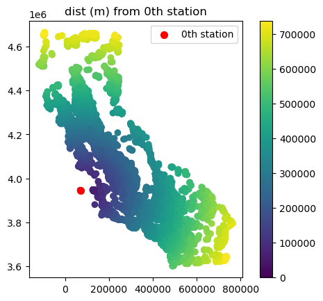
Distances

Similarly, distances between two points can be computed with the distance function:

Let’s calculate the distance between each of the stations in our dataset

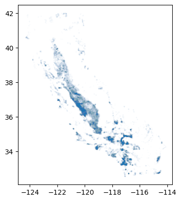
gdf_stns.plot(markersize=1, alpha=0.01)

<Axes: >

# Reproject to UTM zone 11N
gdf_stns.to_crs(gdf_stns.estimate_utm_crs(), inplace=True)

# calculate distance between the first station and each of the other stations
gdf_stns["dist_from_stn_1"] = gdf_stns.distance(gdf_stns.iloc[0].geometry)

# Plot stations, colored by distance
ax = gdf_stns.plot(column="dist_from_stn_1", legend=True)
# Plot the first station in red
gdf_stns.loc[[0], "geometry"].plot(markersize=50, color="red", ax=ax, label="0th station")
# add a legend a title
ax.legend()
ax.set_title("dist (m) from 0th station")

Text(0.5, 1.0, 'dist (m) from 0th station')

Plotting

Just above we see an example of how to color a GeoDataFrame by a column, by specifying the column = 'column_name' argument into gdf.plot().

We can create interactive plots with the gdf.explore() funtion:

gdf_slo = gdf_stns[gdf_stns["COUNTY_NAME"] == "San Luis Obispo"]

gdf_slo.explore(legend=False)

Make this Notebook Trusted to load map: File -> Trust Notebook

Spatial Operations

Geopandas makes it easy to perform basic spatial operations such as Buffers, Convex Hull, and Spatial Joins

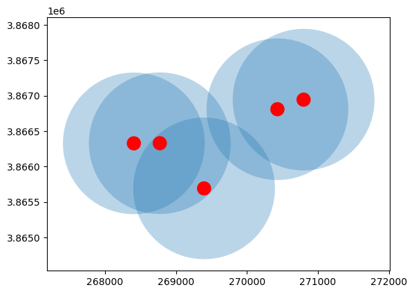
Buffer

# Apply a 1000m buffer to the first 5 points in the SLO well data
ax = gdf_slo[:5].buffer(1000).plot(alpha=0.3)
# Plot the same 5 but with a smaller (100m) buffer
gdf_slo[:5].buffer(100).plot(ax=ax, color="red")

<Axes: >

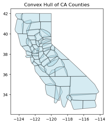
Convex Hull

A convex hull gives the minimum bounds (as polygon) to enclose a number of points or another polygon’s points.

gdf_counties["convex_hull"] = gdf_counties.convex_hull
# Plot the convex hulls
ax = gdf_counties["convex_hull"].plot(alpha=0.5, color="lightblue", edgecolor="black")
ax.set_title("Convex Hull of CA Counties")

Text(0.5, 1.0, 'Convex Hull of CA Counties')

Dissolving Overlapping Polygons

Say we want to create a new single polygon consisting of overlapping polygons, we can achieve this with a dissolve operation

# First we set the geometry column of the gdf to be the buffered polygons instead of the points
gdf_slo_subset = gdf_slo.iloc[:5, :]
gdf_slo_subset.loc[:, "geometry"] = gdf_slo_subset.buffer(1000)
gdf_slo_subset.plot()

<Axes: >

gdf_slo_subset.head()

	STN_ID	SITE_CODE	SWN	WELL_NAME	LATITUDE	LONGITUDE	WLM_METHOD	WLM_ACC	BASIN_CODE	BASIN_NAME	COUNTY_NAME	WELL_DEPTH	WELL_USE	WELL_TYPE	WCR_NO	ZIP_CODE	geometry	dist_from_stn_1
14732	14515	349075N1195236W001	10N25W35F001S	NaN	34.9075	-119.524	Unknown	Unknown	3-013	Cuyama Valley	San Luis Obispo	NaN	Unknown	Unknown	NaN	92154	POLYGON ((270395.988 3865693.001, 270391.173 3...	215821.092758
14834	32411	349130N1195350W001	10N25W27R001S	NaN	34.9130	-119.535	Unknown	Unknown	3-013	Cuyama Valley	San Luis Obispo	NaN	Unknown	Unknown	NaN	92154	POLYGON ((269406.21 3866328.542, 269401.395 38...	214666.454544
14835	38827	349131N1195309W001	10N25W27R002S	NaN	34.9131	-119.531	Unknown	Unknown	3-013	Cuyama Valley	San Luis Obispo	NaN	Unknown	Unknown	NaN	92154	POLYGON ((269772.007 3866330.38, 269767.192 38...	215005.755313
14924	14511	349178N1195134W001	10N25W25M003S	NaN	34.9178	-119.513	Unknown	Unknown	3-013	Cuyama Valley	San Luis Obispo	NaN	Unknown	Unknown	NaN	92154	POLYGON ((271429.923 3866810.295, 271425.107 3...	216372.474901
14942	32409	349191N1195092W001	10N25W25M004S	NaN	34.9191	-119.509	Unknown	Unknown	3-013	Cuyama Valley	San Luis Obispo	NaN	Unknown	Unknown	NaN	92154	POLYGON ((271799.033 3866945.332, 271794.218 3...	216667.216124

gdf_slo_subset.dissolve().plot()

<Axes: >

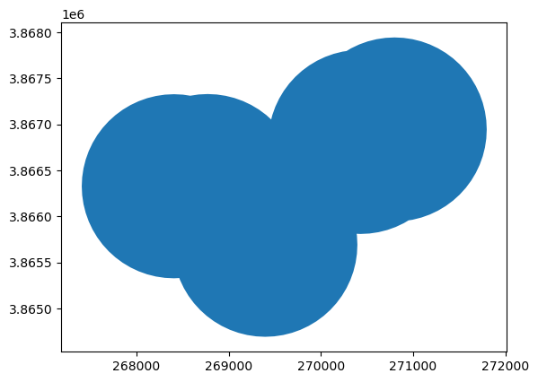
# Notice that there is only one row in the gdf after performing the dissolve
# values are inherited from the first row, but the geometry is the unary_union of all geometryes
gdf_slo_subset.dissolve().head()

	geometry	STN_ID	SITE_CODE	SWN	WELL_NAME	LATITUDE	LONGITUDE	WLM_METHOD	WLM_ACC	BASIN_CODE	BASIN_NAME	COUNTY_NAME	WELL_DEPTH	WELL_USE	WELL_TYPE	WCR_NO	ZIP_CODE	dist_from_stn_1
0	POLYGON ((270376.773 3865497.911, 270352.928 3...	14515	349075N1195236W001	10N25W35F001S	None	34.9075	-119.524	Unknown	Unknown	3-013	Cuyama Valley	San Luis Obispo	NaN	Unknown	Unknown	None	92154	215821.092758

Spatial Joins, Queries, and Relations

Intersections

To check for spatial intersection between two geographic datasets, we can use the intersection function:

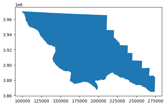
# Check which wells intersect with SLO's geometry
gdf_slo = gdf_counties[gdf_counties["name"] == "San Luis Obispo"].to_crs(gdf_counties.estimate_utm_crs())

gdf_slo.plot()

<Axes: >

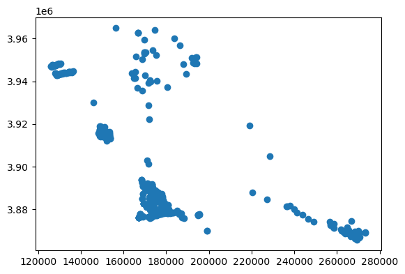
slo_co_stns = gpd.overlay(gdf_stns, gdf_slo, how="intersection")

slo_co_stns.plot()

<Axes: >

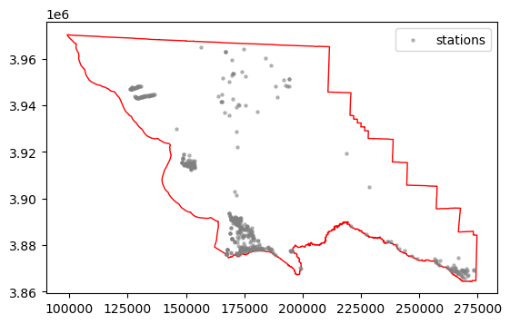
ax = gdf_slo.plot(color="white", edgecolor="red")
slo_co_stns.plot(alpha=0.5, markersize=5, color="gray", label="stations", ax=ax)
ax.legend()

<matplotlib.legend.Legend at 0x16c63cb90>

Exercise

1. Determine how many “Industrial”, “Irrigation”, and “Observation” Wells are in SLO County

2. Create a basic map showing each category as a different color

Rasterio

Rasterio is a powerful library for working with raster data (think: images or grids of numbers with pixels) written on top of the Geospatial Data Abstraction Library (GDAL), that makes it easy to perform a wide variety of raster processing and visualization tasks.

Reading and inspecting data

We can open geospatial raster datasets (e.g. .tif and .tiff files) using the .open function:

import rasterio as rio

# raster_path = "https://github.com/opengeos/datasets/releases/download/raster/dem_90m.tif"
raster_path = "./data/dem_90m.tif"
src = rio.open(raster_path)
print(src)

<open DatasetReader name='./data/dem_90m.tif' mode='r'>

Notice that we are reading a file from a URL here, but this function works identically for local files.

Once a dataset has been opened, we can inspect lots of useful information, including:

• Projection information

• Bounding box

• Spatial resolution

• Dimensions - width / height

• Other metadata

# Inspect crs
src.crs

CRS.from_wkt('PROJCS["WGS 84 / Pseudo-Mercator",GEOGCS["WGS 84",DATUM["WGS_1984",SPHEROID["WGS 84",6378137,298.257223563,AUTHORITY["EPSG","7030"]],AUTHORITY["EPSG","6326"]],PRIMEM["Greenwich",0,AUTHORITY["EPSG","8901"]],UNIT["degree",0.0174532925199433,AUTHORITY["EPSG","9122"]],AUTHORITY["EPSG","4326"]],PROJECTION["Mercator_1SP"],PARAMETER["central_meridian",0],PARAMETER["scale_factor",1],PARAMETER["false_easting",0],PARAMETER["false_northing",0],UNIT["metre",1,AUTHORITY["EPSG","9001"]],AXIS["Easting",EAST],AXIS["Northing",NORTH],EXTENSION["PROJ4","+proj=merc +a=6378137 +b=6378137 +lat_ts=0 +lon_0=0 +x_0=0 +y_0=0 +k=1 +units=m +nadgrids=@null +wktext +no_defs"],AUTHORITY["EPSG","3857"]]')

# Get the EPSG code of the CRS
src.crs.to_epsg()

3857

# Inspect metadata
src.meta

{'driver': 'GTiff',
 'dtype': 'int16',
 'nodata': None,
 'width': 4269,
 'height': 3113,
 'count': 1,
 'crs': CRS.from_wkt('PROJCS["WGS 84 / Pseudo-Mercator",GEOGCS["WGS 84",DATUM["WGS_1984",SPHEROID["WGS 84",6378137,298.257223563,AUTHORITY["EPSG","7030"]],AUTHORITY["EPSG","6326"]],PRIMEM["Greenwich",0,AUTHORITY["EPSG","8901"]],UNIT["degree",0.0174532925199433,AUTHORITY["EPSG","9122"]],AUTHORITY["EPSG","4326"]],PROJECTION["Mercator_1SP"],PARAMETER["central_meridian",0],PARAMETER["scale_factor",1],PARAMETER["false_easting",0],PARAMETER["false_northing",0],UNIT["metre",1,AUTHORITY["EPSG","9001"]],AXIS["Easting",EAST],AXIS["Northing",NORTH],EXTENSION["PROJ4","+proj=merc +a=6378137 +b=6378137 +lat_ts=0 +lon_0=0 +x_0=0 +y_0=0 +k=1 +units=m +nadgrids=@null +wktext +no_defs"],AUTHORITY["EPSG","3857"]]'),
 'transform': Affine(90.0, 0.0, -13442488.3428,
        0.0, -89.99579177642138, 4668371.5775)}

Discussion: What do the dtype, count, and nodata values in the src.meta dict mean?

# Inspect spatial res
src.res

(90.0, 89.99579177642138)

# Inspect dimensions or width / height
print(src.shape, src.width, src.height)

(3113, 4269) 4269 3113

# Inspect bounding box
src.bounds

BoundingBox(left=-13442488.3428, bottom=4388214.6777, right=-13058278.3428, top=4668371.5775)

Plotting and visualizing

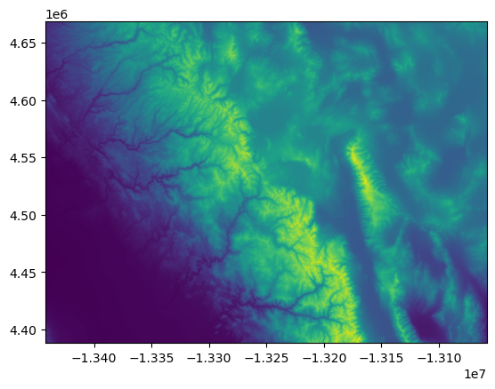
We can use the read function to read raster bands from .tiff or .tif files as numpy arrays, and then make use the imshow function from the trusty module matplotlib!

import numpy as np
import matplotlib.pyplot as plt

arr = src.read(1)
plt.imshow(arr)
plt.colorbar()

<matplotlib.colorbar.Colorbar at 0x1754dafd0>

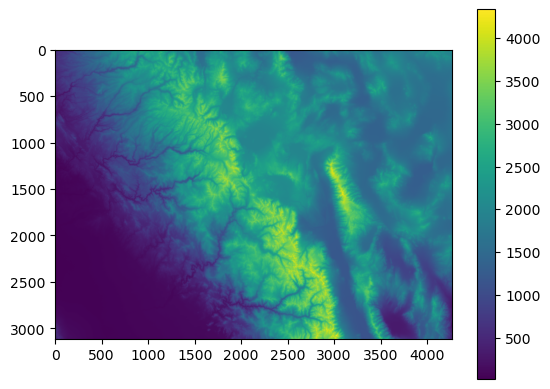
In the above code, we are reading the first band from the raster using src.read(1). For multiband rasters, we can read the other bands using the same syntax.

Note that this method does not preserve any projection information in the plot - the x and y axes are just the number of rows / cols in the dataset.

If we want to preserve any geospatial coordinate information, we can use the rasterio plotting module:

import rasterio.plot

rio.plot.show(src)

<Axes: >

Exercise

• set all values in raster less than 500 equal to np.nan

• Set all values greater than 1000 to np.nan

• Calculate the mean of the remaining raster cells

• Hint - inspect the data type of the array using the arr.dtype syntax, and convert as needed

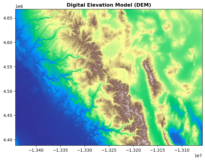
Formatting Plots

We can leverage matplotlib’s functionality to style our plots, including adding titles and choosing colormaps:

fig, ax = plt.subplots(figsize=(8, 8))
rasterio.plot.show(src, cmap="terrain", ax=ax, title="Digital Elevation Model (DEM)")
plt.show()

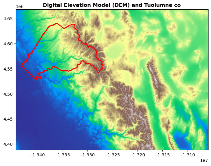
Plotting vector and raster data

Tuolumne_co = gdf_counties[
    gdf_counties["name"] == "Tuolumne"
].copy()  # We need to make a copy of this object to avoid a SettingWithCopyWarning
Tuolumne_co.to_crs(src.crs, inplace=True)

fig, ax = plt.subplots(figsize=(8, 8))
rasterio.plot.show(src, cmap="terrain", ax=ax, title="Digital Elevation Model (DEM) and Tuolumne co")
Tuolumne_co.plot(ax=ax, edgecolor="red", facecolor="none", lw=2)

<Axes: title={'center': 'Digital Elevation Model (DEM) and Tuolumne co'}>

Clipping raster to vector data

A common task involves clipping a raster to a vector dataset. We can use rasterio.mask to clip the DEM above to the boundary of Tuolumne county, defined in the ca_counties.geojson file:

import rasterio.mask

# Read raster
raster_path = "https://github.com/opengeos/datasets/releases/download/raster/dem_90m.tif"
raster_path = "./data/dem_90m.tif"

src = rio.open(raster_path)

# Read shape, isolate Tuolumne
shp_geom = gpd.read_file("ca_counties.geojson")
Tuolumne_co = shp_geom[shp_geom["name"] == "Tuolumne"].copy()  # We need to make a copy of this object to avoid a SettingWithCopyWarning

# Ensure CRS are consistent
Tuolumne_co.to_crs(src.crs, inplace=True)

# Perform clip
out_image, out_transform = rio.mask.mask(src, Tuolumne_co["geometry"], crop=True)

# Verify results:

rasterio.plot.show(out_image[0, :, :]);

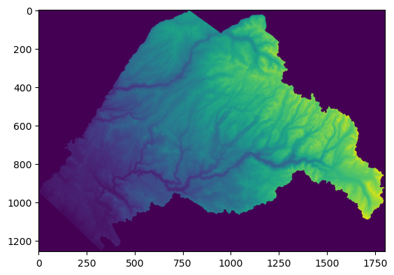
Notice that rasterio returns by default an array with 3 dimensions (out_image), for which we have selected the first band manually. This functionality exists to deal with multiband rasters.

Writing rasters

Let’s save the raster we just clipped

# Set the output file
output_raster_path = "./data/clipped.tif"

# Extract some information from the image we processed
kwargs = src.meta
kwargs.update(height=out_image.shape[1], width=out_image.shape[2], count=out_image.shape[0], dtype=out_image.dtype, crs=src.crs)

# Save
with rasterio.open(output_raster_path, "w", **kwargs) as dst:
    dst.write(out_image)

print(f"Raster data has been written to {output_raster_path}")

Raster data has been written to ./data/clipped.tif

Reprojecting Rasters

We use the rasterio.warp module to change raster projections.

Let’s reproject our clipped raster to the WGS 84 (EPSG:3857) CRS and save the reprojected raster to a new file.

from rasterio.warp import calculate_default_transform, reproject, Resampling

# Set output filename
raster_path = "./data/clipped.tif"
dst_crs = "EPSG:4326"  # WGS 84
output_reprojected_path = "./data/clipped_reprojected.tif"

with rasterio.open(raster_path) as src:
    transform, width, height = calculate_default_transform(src.crs, dst_crs, src.width, src.height, *src.bounds)

    profile = src.profile
    profile.update(crs=dst_crs, transform=transform, width=width, height=height)

    with rasterio.open(output_reprojected_path, "w", **profile) as dst:
        for i in range(1, src.count + 1):
            reproject(
                source=rasterio.band(src, i),
                destination=rasterio.band(dst, i),
                src_transform=src.transform,
                src_crs=src.crs,
                dst_transform=transform,
                dst_crs=dst_crs,
                resampling=Resampling.nearest,
            )
print(f"Reprojected raster saved at {output_reprojected_path}")

Reprojected raster saved at ./data/clipped_reprojected.tif

Multiband Rasters

Satellite data is generally composed of a number of spectral bands. Each band measures the light reflected between two wavelengths (hence the term ‘band’). Rasterio allows us to work with these bands individually and in concert.

For example, NASA’s Landsat Satellites record the following bands:

Name	Wavelength	Description
SR_B1	0.435-0.451 μm	Band 1 (ultra blue, coastal aerosol) surface reflectance
SR_B2	0.452-0.512 μm	Band 2 (blue) surface reflectance
SR_B3	0.533-0.590 μm	Band 3 (green) surface reflectance
SR_B4	0.636-0.673 μm	Band 4 (red) surface reflectance
SR_B5	0.851-0.879 μm	Band 5 (near infrared) surface reflectance
SR_B6	1.566-1.651 μm	Band 6 (shortwave infrared 1) surface reflectance
SR_B7	2.107-2.294 μm	Band 7 (shortwave infrared 2) surface reflectance

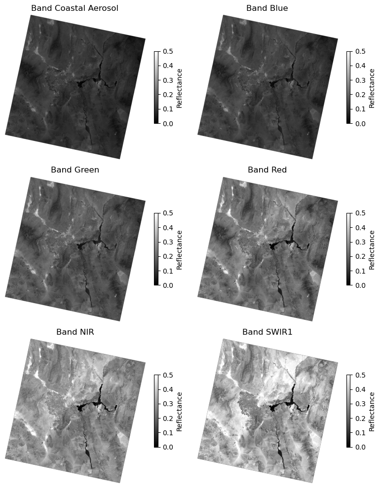
Let’s plot all the bands in this raster

# Read multiband Landsat image:
raster_path = "https://github.com/opengeos/datasets/releases/download/raster/LC09_039035_20240708_90m.tif"
# raster_path = "./data/LC09_039035_20240708_90m.tif"
src = rasterio.open(raster_path)
print(src)

# Specify band names:
band_names = ["Coastal Aerosol", "Blue", "Green", "Red", "NIR", "SWIR1", "SWIR2"]

<open DatasetReader name='https://github.com/opengeos/datasets/releases/download/raster/LC09_039035_20240708_90m.tif' mode='r'>

# Plot raster:

fig, axes = plt.subplots(nrows=3, ncols=2, figsize=(8, 10))
axes = axes.flatten()  # Flatten the 2D array of axes to 1D for easy iteration

for band in range(1, src.count):
    data = src.read(band)
    ax = axes[band - 1]
    im = ax.imshow(data, cmap="gray", vmin=0, vmax=0.5)
    ax.set_title(f"Band {band_names[band - 1]}")
    ax.axis("off")
    fig.colorbar(im, ax=ax, label="Reflectance", shrink=0.5)

plt.tight_layout()
plt.show()

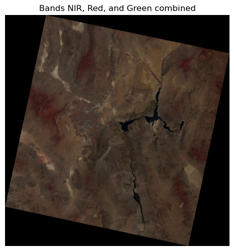
True color image

In order to visualize a true color image, we need to visualize band 2 (blue), band 3 (green), and band 4 (red) in the same image:

nir_band = src.read(5)
red_band = src.read(4)
green_band = src.read(3)

# Stack the bands into a single array
rgb = np.dstack((nir_band, red_band, green_band)).clip(0, 1)

# Plot the stacked array
plt.figure(figsize=(6, 6))
plt.imshow(rgb)
plt.axis("off")
plt.title("Bands NIR, Red, and Green combined")
plt.show()

src.nodata

-inf

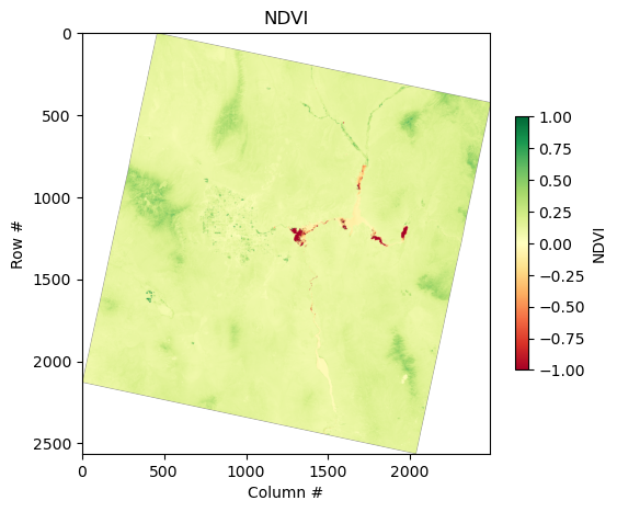
Band math: Calculating NDVI

A common metric that we can derive from multiple bands is Normalized Difference Vegetation Index (NDVI), which is defined as:

\[NDVI = (NIR - Red) / (NIR + Red)\]

# NDVI Calculation: NDVI = (NIR - Red) / (NIR + Red)
ndvi = (nir_band - red_band) / (nir_band + red_band)

/var/folders/df/w347rlh96tx42h1kl69_4r8w0000gn/T/ipykernel_73601/134765836.py:2: RuntimeWarning: invalid value encountered in subtract
  ndvi = (nir_band - red_band) / (nir_band + red_band)

We received a RuntimeWarning about invalid values in our subtract operation. This is likely due to the ‘no data’ areas denoted by the black pixels in the true color image above. We can read the nodata value directly from rasterio and use numpy to change the nodata values in order to fix this issue:

# Set the nodata value to numpy nan for each of the bands
nir_band[nir_band == src.nodata] = np.nan
red_band[red_band == src.nodata] = np.nan

# NDVI Calculation: NDVI = (NIR - Red) / (NIR + Red)
ndvi = (nir_band - red_band) / (nir_band + red_band)
ndvi = ndvi.clip(-1, 1)

plt.figure(figsize=(6, 6))
plt.imshow(ndvi, cmap="RdYlGn", vmin=-1, vmax=1)
plt.colorbar(label="NDVI", shrink=0.5)
plt.title("NDVI")
plt.xlabel("Column #")
plt.ylabel("Row #")
plt.show()

Xarray

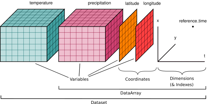
Xarray makes working with labelled multi-dimensional arrays in Python simple, efficient, and fun!

Xarray extends NumPy functionality by providing data structures specifically for geospatial multi-dimensional arrays:

DataArray: A labeled, multi-dimensional array, which includes dimensions, coordinates, and attributes.

Dataset: A collection of DataArray objects that share the same dimensions.

Xarray data representation

Xarray represents stacks of images as ‘cubes’, where two axes represent the latitude and longitude coordinates of spatial data, and a third axis represents time. Note that an xarray dataset can contain more than one variable!

The schematic below shows examples for temperature and precipitation

Loading Data and inspecting attributes

This data was downloaded from NOAA: https://psl.noaa.gov/data/gridded/data.ncep.reanalysis.html

import xarray as xr

ds = xr.open_dataset("./data/runof.sfc.mon.mean.nc")
ds

<xarray.Dataset> Size: 67MB
Dimensions:  (lat: 94, lon: 192, time: 923)
Coordinates:
  * lat      (lat) float32 376B 88.54 86.65 84.75 82.85 ... -84.75 -86.65 -88.54
  * lon      (lon) float32 768B 0.0 1.875 3.75 5.625 ... 352.5 354.4 356.2 358.1
  * time     (time) datetime64[ns] 7kB 1948-01-01 1948-02-01 ... 2024-11-01
Data variables:
    runof    (time, lat, lon) float32 67MB ...
Attributes:
    description:    Data is from NMC initialized reanalysis\n(4x/day).  It co...
    platform:       Model
    Conventions:    COARDS
    NCO:            20121013
    history:        Mon Jul  5 23:58:07 1999: ncrcat runof.mon.mean.nc /Datas...
    title:          monthly mean runof.sfc from the NCEP Reanalysis
    dataset_title:  NCEP-NCAR Reanalysis 1
    References:     http://www.psl.noaa.gov/data/gridded/data.ncep.reanalysis...

xarray.Dataset

• Dimensions:
  • lat: 94
  • lon: 192
  • time: 923
• Coordinates: (3)
  • lat
    (lat)
    float32
    88.54 86.65 84.75 ... -86.65 -88.54

    units :

    degrees_north

    actual_range :

    [ 88.542 -88.542]

    long_name :

    Latitude

    standard_name :

    latitude

    axis :

    Y

    array([ 88.542   ,  86.6531  ,  84.7532  ,  82.8508  ,  80.9473  ,  79.0435  ,
            77.1394  ,  75.2351  ,  73.3307  ,  71.4262  ,  69.5217  ,  67.6171  ,
            65.7125  ,  63.8079  ,  61.9033  ,  59.9986  ,  58.0939  ,  56.1893  ,
            54.2846  ,  52.3799  ,  50.4752  ,  48.5705  ,  46.6658  ,  44.7611  ,
            42.8564  ,  40.9517  ,  39.047   ,  37.1422  ,  35.2375  ,  33.3328  ,
            31.4281  ,  29.5234  ,  27.6186  ,  25.7139  ,  23.8092  ,  21.9044  ,
            19.9997  ,  18.095   ,  16.1902  ,  14.2855  ,  12.3808  ,  10.47604 ,
             8.57131 ,   6.66657 ,   4.76184 ,   2.8571  ,   0.952368,  -0.952368,
            -2.8571  ,  -4.76184 ,  -6.66657 ,  -8.57131 , -10.47604 , -12.3808  ,
           -14.2855  , -16.1902  , -18.095   , -19.9997  , -21.9044  , -23.8092  ,
           -25.7139  , -27.6186  , -29.5234  , -31.4281  , -33.3328  , -35.2375  ,
           -37.1422  , -39.047   , -40.9517  , -42.8564  , -44.7611  , -46.6658  ,
           -48.5705  , -50.4752  , -52.3799  , -54.2846  , -56.1893  , -58.0939  ,
           -59.9986  , -61.9033  , -63.8079  , -65.7125  , -67.6171  , -69.5217  ,
           -71.4262  , -73.3307  , -75.2351  , -77.1394  , -79.0435  , -80.9473  ,
           -82.8508  , -84.7532  , -86.6531  , -88.542   ], dtype=float32)

  • lon
    (lon)
    float32
    0.0 1.875 3.75 ... 356.2 358.1

    units :

    degrees_east

    long_name :

    Longitude

    actual_range :

    [ 0. 358.125]

    standard_name :

    longitude

    axis :

    X

    array([  0.   ,   1.875,   3.75 ,   5.625,   7.5  ,   9.375,  11.25 ,  13.125,
            15.   ,  16.875,  18.75 ,  20.625,  22.5  ,  24.375,  26.25 ,  28.125,
            30.   ,  31.875,  33.75 ,  35.625,  37.5  ,  39.375,  41.25 ,  43.125,
            45.   ,  46.875,  48.75 ,  50.625,  52.5  ,  54.375,  56.25 ,  58.125,
            60.   ,  61.875,  63.75 ,  65.625,  67.5  ,  69.375,  71.25 ,  73.125,
            75.   ,  76.875,  78.75 ,  80.625,  82.5  ,  84.375,  86.25 ,  88.125,
            90.   ,  91.875,  93.75 ,  95.625,  97.5  ,  99.375, 101.25 , 103.125,
           105.   , 106.875, 108.75 , 110.625, 112.5  , 114.375, 116.25 , 118.125,
           120.   , 121.875, 123.75 , 125.625, 127.5  , 129.375, 131.25 , 133.125,
           135.   , 136.875, 138.75 , 140.625, 142.5  , 144.375, 146.25 , 148.125,
           150.   , 151.875, 153.75 , 155.625, 157.5  , 159.375, 161.25 , 163.125,
           165.   , 166.875, 168.75 , 170.625, 172.5  , 174.375, 176.25 , 178.125,
           180.   , 181.875, 183.75 , 185.625, 187.5  , 189.375, 191.25 , 193.125,
           195.   , 196.875, 198.75 , 200.625, 202.5  , 204.375, 206.25 , 208.125,
           210.   , 211.875, 213.75 , 215.625, 217.5  , 219.375, 221.25 , 223.125,
           225.   , 226.875, 228.75 , 230.625, 232.5  , 234.375, 236.25 , 238.125,
           240.   , 241.875, 243.75 , 245.625, 247.5  , 249.375, 251.25 , 253.125,
           255.   , 256.875, 258.75 , 260.625, 262.5  , 264.375, 266.25 , 268.125,
           270.   , 271.875, 273.75 , 275.625, 277.5  , 279.375, 281.25 , 283.125,
           285.   , 286.875, 288.75 , 290.625, 292.5  , 294.375, 296.25 , 298.125,
           300.   , 301.875, 303.75 , 305.625, 307.5  , 309.375, 311.25 , 313.125,
           315.   , 316.875, 318.75 , 320.625, 322.5  , 324.375, 326.25 , 328.125,
           330.   , 331.875, 333.75 , 335.625, 337.5  , 339.375, 341.25 , 343.125,
           345.   , 346.875, 348.75 , 350.625, 352.5  , 354.375, 356.25 , 358.125],
          dtype=float32)

  • time
    (time)
    datetime64[ns]
    1948-01-01 ... 2024-11-01

    long_name :

    Time

    delta_t :

    0000-01-00 00:00:00

    avg_period :

    0000-01-00 00:00:00

    prev_avg_period :

    0000-00-01 00:00:00

    standard_name :

    time

    axis :

    T

    actual_range :

    [1297320. 1970856.]

    array(['1948-01-01T00:00:00.000000000', '1948-02-01T00:00:00.000000000',
           '1948-03-01T00:00:00.000000000', ..., '2024-09-01T00:00:00.000000000',
           '2024-10-01T00:00:00.000000000', '2024-11-01T00:00:00.000000000'],
          shape=(923,), dtype='datetime64[ns]')

• Data variables: (1)
  • runof
    (time, lat, lon)
    float32
    ...

    long_name :

    Monthly Mean of Water Runoff

    valid_range :

    [-400. 700.]

    units :

    kg/m^2

    precision :

    1

    var_desc :

    Water Runoff

    level_desc :

    Surface

    statistic :

    Mean

    parent_stat :

    Individual Obs

    dataset :

    NCEP Reanalysis Derived Products

    actual_range :

    [-5.e+00 1.e+30]

    [16658304 values with dtype=float32]

• Indexes: (3)
  • lat
    PandasIndex

    PandasIndex(Index([  88.54199981689453,    86.6530990600586,    84.7531967163086,
             82.85079956054688,   80.94730377197266,   79.04350280761719,
             77.13939666748047,   75.23509979248047,   73.33070373535156,
             71.42620086669922,   69.52169799804688,   67.61710357666016,
              65.7125015258789,  63.807899475097656,   61.90330123901367,
            59.998600006103516,   58.09389877319336,  56.189300537109375,
             54.28459930419922,   52.37990188598633,   50.47520065307617,
            48.570499420166016,   46.66579818725586,   44.76110076904297,
             42.85639953613281,  40.951698303222656,  39.047000885009766,
              37.1422004699707,   35.23749923706055,  33.332801818847656,
              31.4281005859375,  29.523399353027344,  27.618600845336914,
            25.713899612426758,  23.809200286865234,  21.904399871826172,
             19.99970054626465,  18.094999313354492,  16.190200805664062,
            14.285499572753906,  12.380800247192383,   10.47603988647461,
             8.571310043334961,    6.66657018661499,   4.761839866638184,
             2.857100009918213,  0.9523680210113525, -0.9523680210113525,
            -2.857100009918213,  -4.761839866638184,   -6.66657018661499,
            -8.571310043334961,  -10.47603988647461, -12.380800247192383,
           -14.285499572753906, -16.190200805664062, -18.094999313354492,
            -19.99970054626465, -21.904399871826172, -23.809200286865234,
           -25.713899612426758, -27.618600845336914, -29.523399353027344,
             -31.4281005859375, -33.332801818847656,  -35.23749923706055,
             -37.1422004699707, -39.047000885009766, -40.951698303222656,
            -42.85639953613281,  -44.76110076904297,  -46.66579818725586,
           -48.570499420166016,  -50.47520065307617,  -52.37990188598633,
            -54.28459930419922, -56.189300537109375,  -58.09389877319336,
           -59.998600006103516,  -61.90330123901367, -63.807899475097656,
             -65.7125015258789,  -67.61710357666016,  -69.52169799804688,
            -71.42620086669922,  -73.33070373535156,  -75.23509979248047,
            -77.13939666748047,  -79.04350280761719,  -80.94730377197266,
            -82.85079956054688,   -84.7531967163086,   -86.6530990600586,
            -88.54199981689453],
          dtype='float32', name='lat'))

  • lon
    PandasIndex

    PandasIndex(Index([    0.0,   1.875,    3.75,   5.625,     7.5,   9.375,   11.25,  13.125,
              15.0,  16.875,
           ...
            341.25, 343.125,   345.0, 346.875,  348.75, 350.625,   352.5, 354.375,
            356.25, 358.125],
          dtype='float32', name='lon', length=192))

  • time
    PandasIndex

    PandasIndex(DatetimeIndex(['1948-01-01', '1948-02-01', '1948-03-01', '1948-04-01',
                   '1948-05-01', '1948-06-01', '1948-07-01', '1948-08-01',
                   '1948-09-01', '1948-10-01',
                   ...
                   '2024-02-01', '2024-03-01', '2024-04-01', '2024-05-01',
                   '2024-06-01', '2024-07-01', '2024-08-01', '2024-09-01',
                   '2024-10-01', '2024-11-01'],
                  dtype='datetime64[ns]', name='time', length=923, freq=None))

• Attributes: (8)

  description :

  Data is from NMC initialized reanalysis (4x/day). It consists of T42 variables interpolated to pressure surfaces from model (sigma) surfaces.

  platform :

  Model

  Conventions :

  COARDS

  NCO :

  20121013

  history :

  Mon Jul 5 23:58:07 1999: ncrcat runof.mon.mean.nc /Datasets/ncep.reanalysis.derived/surface_gauss/runof.mon.mean.nc /dm/dmwork/nmc.rean.ingest/combinedMMs/runof.mon.mean.nc runof.sfc.gauss.85.nc created 95/03/13 by Hoop (netCDF2.3) Converted to chunked, deflated non-packed NetCDF4 2014/09

  title :

  monthly mean runof.sfc from the NCEP Reanalysis

  dataset_title :

  NCEP-NCAR Reanalysis 1

  References :

  http://www.psl.noaa.gov/data/gridded/data.ncep.reanalysis.derived.html

ds["runof"].mean(dim="time").plot()

<matplotlib.collections.QuadMesh at 0x38e041090>

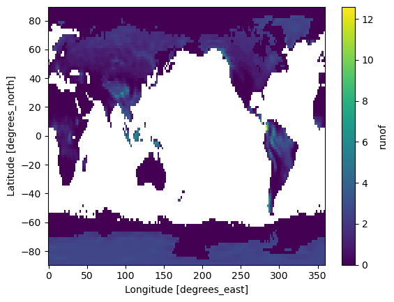
# Select the data array describing runoff
ro = ds["runof"]

# Plot some of the data array attributes

# Obtain a numpy array of the values
print(ro.values.shape)
print(ro.values)

(923, 94, 192)
[[[      nan       nan       nan ...       nan       nan       nan]
  [      nan       nan       nan ...       nan       nan       nan]
  [      nan       nan       nan ...       nan       nan       nan]
  ...
  [1.1632297 1.1696817 1.1729066 ... 1.1600037 1.1600037 1.1600037]
  [1.1600037 1.1600037 1.1600037 ... 1.1600037 1.1600037 1.1600037]
  [1.1729066 1.1761327 1.1790358 ... 1.1696817 1.1696817 1.1729066]]

 [[      nan       nan       nan ...       nan       nan       nan]
  [      nan       nan       nan ...       nan       nan       nan]
  [      nan       nan       nan ...       nan       nan       nan]
  ...
  [1.5599976 1.5599976 1.5599976 ... 1.4944816 1.5186188 1.5427573]
  [1.5389636 1.5389636 1.5389636 ... 1.5358603 1.5358603 1.5389636]
  [1.5599976 1.5599976 1.5599976 ... 1.5599976 1.5599976 1.5599976]]

 [[      nan       nan       nan ...       nan       nan       nan]
  [      nan       nan       nan ...       nan       nan       nan]
  [      nan       nan       nan ...       nan       nan       nan]
  ...
  [1.5599976 1.5599976 1.5599976 ... 1.5599976 1.5599976 1.5599976]
  [1.5599976 1.5599976 1.5599976 ... 1.5599976 1.5599976 1.5599976]
  [1.5599976 1.5599976 1.5599976 ... 1.5599976 1.5599976 1.5599976]]

 ...

 [[0.        0.        0.        ... 0.        0.        0.       ]
  [0.        0.        0.        ... 0.        0.        0.       ]
  [0.        0.        0.        ... 0.        0.        0.       ]
  ...
  [2.8000002 2.9566665 3.1999993 ... 2.8000002 2.8000002 2.8000002]
  [2.8000002 2.8000002 2.8000002 ... 2.8000002 2.8000002 2.8000002]
  [2.8000002 2.8000002 2.8000002 ... 2.8000002 2.8000002 2.8000002]]

 [[0.        0.        0.        ... 0.        0.        0.       ]
  [0.        0.        0.        ... 0.        0.        0.       ]
  [0.        0.        0.        ... 0.        0.        0.       ]
  ...
  [2.8000004 2.8000004 3.0354831 ... 2.8000004 2.8000004 2.8000004]
  [2.8000004 2.8000004 2.8000004 ... 2.8000004 2.8000004 2.8000004]
  [2.8000004 2.8000004 2.8000004 ... 2.8000004 2.8000004 2.8000004]]

 [[0.        0.        0.        ... 0.        0.        0.       ]
  [0.        0.        0.        ... 0.        0.        0.       ]
  [0.        0.        0.        ... 0.        0.        0.       ]
  ...
  [2.8000002 2.8000002 2.8000002 ... 2.8000002 2.8000002 2.8000002]
  [2.8000002 2.8000002 2.8000002 ... 2.8000002 2.8000002 2.8000002]
  [2.8000002 2.8000002 2.8000002 ... 2.8000002 2.8000002 2.8000002]]]

print(ro.coords)

Coordinates:
  * lat      (lat) float32 376B 88.54 86.65 84.75 82.85 ... -84.75 -86.65 -88.54
  * lon      (lon) float32 768B 0.0 1.875 3.75 5.625 ... 352.5 354.4 356.2 358.1
  * time     (time) datetime64[ns] 7kB 1948-01-01 1948-02-01 ... 2024-11-01

print(ro.attrs)

{'long_name': 'Monthly Mean of Water Runoff', 'valid_range': array([-400.,  700.], dtype=float32), 'units': 'kg/m^2', 'precision': np.int16(1), 'var_desc': 'Water Runoff', 'level_desc': 'Surface', 'statistic': 'Mean', 'parent_stat': 'Individual Obs', 'dataset': 'NCEP Reanalysis Derived Products', 'actual_range': array([-5.e+00,  1.e+30], dtype=float32)}

print(ro.dims)

('time', 'lat', 'lon')

Filtering and subsetting

We can easily select data based on dimension labels, which is very intuitive when working with geospatial data.

# Select data for a specific time and location
selected_data = ro.sel(time="2000-01-01", lat=40.0, lon=120.0, method="nearest")
selected_data

<xarray.DataArray 'runof' ()> Size: 4B
array(1.587088, dtype=float32)
Coordinates:
    lat      float32 4B 40.95
    lon      float32 4B 120.0
    time     datetime64[ns] 8B 2000-01-01
Attributes:
    long_name:     Monthly Mean of Water Runoff
    valid_range:   [-400.  700.]
    units:         kg/m^2
    precision:     1
    var_desc:      Water Runoff
    level_desc:    Surface
    statistic:     Mean
    parent_stat:   Individual Obs
    dataset:       NCEP Reanalysis Derived Products
    actual_range:  [-5.e+00  1.e+30]

xarray.DataArray

'runof'

• 1.587

  array(1.587088, dtype=float32)

• Coordinates: (3)
  • lat
    ()
    float32
    40.95

    units :

    degrees_north

    actual_range :

    [ 88.542 -88.542]

    long_name :

    Latitude

    standard_name :

    latitude

    axis :

    Y

    array(40.9517, dtype=float32)

  • lon
    ()
    float32
    120.0

    units :

    degrees_east

    long_name :

    Longitude

    actual_range :

    [ 0. 358.125]

    standard_name :

    longitude

    axis :

    X

    array(120., dtype=float32)

  • time
    ()
    datetime64[ns]
    2000-01-01

    long_name :

    Time

    delta_t :

    0000-01-00 00:00:00

    avg_period :

    0000-01-00 00:00:00

    prev_avg_period :

    0000-00-01 00:00:00

    standard_name :

    time

    axis :

    T

    actual_range :

    [1297320. 1970856.]

    array('2000-01-01T00:00:00.000000000', dtype='datetime64[ns]')

• Indexes: (0)
• Attributes: (10)

  long_name :

  Monthly Mean of Water Runoff

  valid_range :

  [-400. 700.]

  units :

  kg/m^2

  precision :

  1

  var_desc :

  Water Runoff

  level_desc :

  Surface

  statistic :

  Mean

  parent_stat :

  Individual Obs

  dataset :

  NCEP Reanalysis Derived Products

  actual_range :

  [-5.e+00 1.e+30]

# Slice data across a range of times
time_slice = ro.sel(time=slice("2013-01-01", "2013-01-31"))
time_slice

<xarray.DataArray 'runof' (time: 1, lat: 94, lon: 192)> Size: 72kB
array([[[0.      , 0.      , ..., 0.      , 0.      ],
        [0.      , 0.      , ..., 0.      , 0.      ],
        ...,
        [2.580681, 2.590358, ..., 2.567777, 2.574229],
        [2.800049, 2.800049, ..., 2.800049, 2.800049]]],
      shape=(1, 94, 192), dtype=float32)
Coordinates:
  * lat      (lat) float32 376B 88.54 86.65 84.75 82.85 ... -84.75 -86.65 -88.54
  * lon      (lon) float32 768B 0.0 1.875 3.75 5.625 ... 352.5 354.4 356.2 358.1
  * time     (time) datetime64[ns] 8B 2013-01-01
Attributes:
    long_name:     Monthly Mean of Water Runoff
    valid_range:   [-400.  700.]
    units:         kg/m^2
    precision:     1
    var_desc:      Water Runoff
    level_desc:    Surface
    statistic:     Mean
    parent_stat:   Individual Obs
    dataset:       NCEP Reanalysis Derived Products
    actual_range:  [-5.e+00  1.e+30]

xarray.DataArray

'runof'

• time: 1
• lat: 94
• lon: 192

• 0.0 0.0 0.0 0.0 0.0 0.0 0.0 0.0 ... 2.8 2.8 2.8 2.8 2.8 2.8 2.8 2.8

  array([[[0.      , 0.      , ..., 0.      , 0.      ],
          [0.      , 0.      , ..., 0.      , 0.      ],
          ...,
          [2.580681, 2.590358, ..., 2.567777, 2.574229],
          [2.800049, 2.800049, ..., 2.800049, 2.800049]]],
        shape=(1, 94, 192), dtype=float32)

• Coordinates: (3)
  • lat
    (lat)
    float32
    88.54 86.65 84.75 ... -86.65 -88.54

    units :

    degrees_north

    actual_range :

    [ 88.542 -88.542]

    long_name :

    Latitude

    standard_name :

    latitude

    axis :

    Y

    array([ 88.542   ,  86.6531  ,  84.7532  ,  82.8508  ,  80.9473  ,  79.0435  ,
            77.1394  ,  75.2351  ,  73.3307  ,  71.4262  ,  69.5217  ,  67.6171  ,
            65.7125  ,  63.8079  ,  61.9033  ,  59.9986  ,  58.0939  ,  56.1893  ,
            54.2846  ,  52.3799  ,  50.4752  ,  48.5705  ,  46.6658  ,  44.7611  ,
            42.8564  ,  40.9517  ,  39.047   ,  37.1422  ,  35.2375  ,  33.3328  ,
            31.4281  ,  29.5234  ,  27.6186  ,  25.7139  ,  23.8092  ,  21.9044  ,
            19.9997  ,  18.095   ,  16.1902  ,  14.2855  ,  12.3808  ,  10.47604 ,
             8.57131 ,   6.66657 ,   4.76184 ,   2.8571  ,   0.952368,  -0.952368,
            -2.8571  ,  -4.76184 ,  -6.66657 ,  -8.57131 , -10.47604 , -12.3808  ,
           -14.2855  , -16.1902  , -18.095   , -19.9997  , -21.9044  , -23.8092  ,
           -25.7139  , -27.6186  , -29.5234  , -31.4281  , -33.3328  , -35.2375  ,
           -37.1422  , -39.047   , -40.9517  , -42.8564  , -44.7611  , -46.6658  ,
           -48.5705  , -50.4752  , -52.3799  , -54.2846  , -56.1893  , -58.0939  ,
           -59.9986  , -61.9033  , -63.8079  , -65.7125  , -67.6171  , -69.5217  ,
           -71.4262  , -73.3307  , -75.2351  , -77.1394  , -79.0435  , -80.9473  ,
           -82.8508  , -84.7532  , -86.6531  , -88.542   ], dtype=float32)

  • lon
    (lon)
    float32
    0.0 1.875 3.75 ... 356.2 358.1

    units :

    degrees_east

    long_name :

    Longitude

    actual_range :

    [ 0. 358.125]

    standard_name :

    longitude

    axis :

    X

    array([  0.   ,   1.875,   3.75 ,   5.625,   7.5  ,   9.375,  11.25 ,  13.125,
            15.   ,  16.875,  18.75 ,  20.625,  22.5  ,  24.375,  26.25 ,  28.125,
            30.   ,  31.875,  33.75 ,  35.625,  37.5  ,  39.375,  41.25 ,  43.125,
            45.   ,  46.875,  48.75 ,  50.625,  52.5  ,  54.375,  56.25 ,  58.125,
            60.   ,  61.875,  63.75 ,  65.625,  67.5  ,  69.375,  71.25 ,  73.125,
            75.   ,  76.875,  78.75 ,  80.625,  82.5  ,  84.375,  86.25 ,  88.125,
            90.   ,  91.875,  93.75 ,  95.625,  97.5  ,  99.375, 101.25 , 103.125,
           105.   , 106.875, 108.75 , 110.625, 112.5  , 114.375, 116.25 , 118.125,
           120.   , 121.875, 123.75 , 125.625, 127.5  , 129.375, 131.25 , 133.125,
           135.   , 136.875, 138.75 , 140.625, 142.5  , 144.375, 146.25 , 148.125,
           150.   , 151.875, 153.75 , 155.625, 157.5  , 159.375, 161.25 , 163.125,
           165.   , 166.875, 168.75 , 170.625, 172.5  , 174.375, 176.25 , 178.125,
           180.   , 181.875, 183.75 , 185.625, 187.5  , 189.375, 191.25 , 193.125,
           195.   , 196.875, 198.75 , 200.625, 202.5  , 204.375, 206.25 , 208.125,
           210.   , 211.875, 213.75 , 215.625, 217.5  , 219.375, 221.25 , 223.125,
           225.   , 226.875, 228.75 , 230.625, 232.5  , 234.375, 236.25 , 238.125,
           240.   , 241.875, 243.75 , 245.625, 247.5  , 249.375, 251.25 , 253.125,
           255.   , 256.875, 258.75 , 260.625, 262.5  , 264.375, 266.25 , 268.125,
           270.   , 271.875, 273.75 , 275.625, 277.5  , 279.375, 281.25 , 283.125,
           285.   , 286.875, 288.75 , 290.625, 292.5  , 294.375, 296.25 , 298.125,
           300.   , 301.875, 303.75 , 305.625, 307.5  , 309.375, 311.25 , 313.125,
           315.   , 316.875, 318.75 , 320.625, 322.5  , 324.375, 326.25 , 328.125,
           330.   , 331.875, 333.75 , 335.625, 337.5  , 339.375, 341.25 , 343.125,
           345.   , 346.875, 348.75 , 350.625, 352.5  , 354.375, 356.25 , 358.125],
          dtype=float32)

  • time
    (time)
    datetime64[ns]
    2013-01-01

    long_name :

    Time

    delta_t :

    0000-01-00 00:00:00

    avg_period :

    0000-01-00 00:00:00

    prev_avg_period :

    0000-00-01 00:00:00

    standard_name :

    time

    axis :

    T

    actual_range :

    [1297320. 1970856.]

    array(['2013-01-01T00:00:00.000000000'], dtype='datetime64[ns]')

• Indexes: (3)
  • lat
    PandasIndex

    PandasIndex(Index([  88.54199981689453,    86.6530990600586,    84.7531967163086,
             82.85079956054688,   80.94730377197266,   79.04350280761719,
             77.13939666748047,   75.23509979248047,   73.33070373535156,
             71.42620086669922,   69.52169799804688,   67.61710357666016,
              65.7125015258789,  63.807899475097656,   61.90330123901367,
            59.998600006103516,   58.09389877319336,  56.189300537109375,
             54.28459930419922,   52.37990188598633,   50.47520065307617,
            48.570499420166016,   46.66579818725586,   44.76110076904297,
             42.85639953613281,  40.951698303222656,  39.047000885009766,
              37.1422004699707,   35.23749923706055,  33.332801818847656,
              31.4281005859375,  29.523399353027344,  27.618600845336914,
            25.713899612426758,  23.809200286865234,  21.904399871826172,
             19.99970054626465,  18.094999313354492,  16.190200805664062,
            14.285499572753906,  12.380800247192383,   10.47603988647461,
             8.571310043334961,    6.66657018661499,   4.761839866638184,
             2.857100009918213,  0.9523680210113525, -0.9523680210113525,
            -2.857100009918213,  -4.761839866638184,   -6.66657018661499,
            -8.571310043334961,  -10.47603988647461, -12.380800247192383,
           -14.285499572753906, -16.190200805664062, -18.094999313354492,
            -19.99970054626465, -21.904399871826172, -23.809200286865234,
           -25.713899612426758, -27.618600845336914, -29.523399353027344,
             -31.4281005859375, -33.332801818847656,  -35.23749923706055,
             -37.1422004699707, -39.047000885009766, -40.951698303222656,
            -42.85639953613281,  -44.76110076904297,  -46.66579818725586,
           -48.570499420166016,  -50.47520065307617,  -52.37990188598633,
            -54.28459930419922, -56.189300537109375,  -58.09389877319336,
           -59.998600006103516,  -61.90330123901367, -63.807899475097656,
             -65.7125015258789,  -67.61710357666016,  -69.52169799804688,
            -71.42620086669922,  -73.33070373535156,  -75.23509979248047,
            -77.13939666748047,  -79.04350280761719,  -80.94730377197266,
            -82.85079956054688,   -84.7531967163086,   -86.6530990600586,
            -88.54199981689453],
          dtype='float32', name='lat'))

  • lon
    PandasIndex

    PandasIndex(Index([    0.0,   1.875,    3.75,   5.625,     7.5,   9.375,   11.25,  13.125,
              15.0,  16.875,
           ...
            341.25, 343.125,   345.0, 346.875,  348.75, 350.625,   352.5, 354.375,
            356.25, 358.125],
          dtype='float32', name='lon', length=192))

  • time
    PandasIndex

    PandasIndex(DatetimeIndex(['2013-01-01'], dtype='datetime64[ns]', name='time', freq=None))

• Attributes: (10)

  long_name :

  Monthly Mean of Water Runoff

  valid_range :

  [-400. 700.]

  units :

  kg/m^2

  precision :

  1

  var_desc :

  Water Runoff

  level_desc :

  Surface

  statistic :

  Mean

  parent_stat :

  Individual Obs

  dataset :

  NCEP Reanalysis Derived Products

  actual_range :

  [-5.e+00 1.e+30]

# Calculate the mean SWE over time
mean_ro = ro.mean(dim="time")
mean_ro

<xarray.DataArray 'runof' (lat: 94, lon: 192)> Size: 72kB
array([[0.       , 0.       , 0.       , ..., 0.       , 0.       ,
        0.       ],
       [0.       , 0.       , 0.       , ..., 0.       , 0.       ,
        0.       ],
       [0.       , 0.       , 0.       , ..., 0.       , 0.       ,
        0.       ],
       ...,
       [2.635003 , 2.6681736, 2.7444425, ..., 2.6152654, 2.6228926,
        2.6288702],
       [2.6165829, 2.6178818, 2.6189005, ..., 2.6109586, 2.6131048,
        2.6150517],
       [2.6433473, 2.6445358, 2.645743 , ..., 2.6407027, 2.641557 ,
        2.6424491]], shape=(94, 192), dtype=float32)
Coordinates:
  * lat      (lat) float32 376B 88.54 86.65 84.75 82.85 ... -84.75 -86.65 -88.54
  * lon      (lon) float32 768B 0.0 1.875 3.75 5.625 ... 352.5 354.4 356.2 358.1

xarray.DataArray

'runof'

• lat: 94
• lon: 192

• 0.0 0.0 0.0 0.0 0.0 0.0 0.0 ... 2.638 2.639 2.64 2.641 2.642 2.642

  array([[0.       , 0.       , 0.       , ..., 0.       , 0.       ,
          0.       ],
         [0.       , 0.       , 0.       , ..., 0.       , 0.       ,
          0.       ],
         [0.       , 0.       , 0.       , ..., 0.       , 0.       ,
          0.       ],
         ...,
         [2.635003 , 2.6681736, 2.7444425, ..., 2.6152654, 2.6228926,
          2.6288702],
         [2.6165829, 2.6178818, 2.6189005, ..., 2.6109586, 2.6131048,
          2.6150517],
         [2.6433473, 2.6445358, 2.645743 , ..., 2.6407027, 2.641557 ,
          2.6424491]], shape=(94, 192), dtype=float32)

• Coordinates: (2)
  • lat
    (lat)
    float32
    88.54 86.65 84.75 ... -86.65 -88.54

    units :

    degrees_north

    actual_range :

    [ 88.542 -88.542]

    long_name :

    Latitude

    standard_name :

    latitude

    axis :

    Y

    array([ 88.542   ,  86.6531  ,  84.7532  ,  82.8508  ,  80.9473  ,  79.0435  ,
            77.1394  ,  75.2351  ,  73.3307  ,  71.4262  ,  69.5217  ,  67.6171  ,
            65.7125  ,  63.8079  ,  61.9033  ,  59.9986  ,  58.0939  ,  56.1893  ,
            54.2846  ,  52.3799  ,  50.4752  ,  48.5705  ,  46.6658  ,  44.7611  ,
            42.8564  ,  40.9517  ,  39.047   ,  37.1422  ,  35.2375  ,  33.3328  ,
            31.4281  ,  29.5234  ,  27.6186  ,  25.7139  ,  23.8092  ,  21.9044  ,
            19.9997  ,  18.095   ,  16.1902  ,  14.2855  ,  12.3808  ,  10.47604 ,
             8.57131 ,   6.66657 ,   4.76184 ,   2.8571  ,   0.952368,  -0.952368,
            -2.8571  ,  -4.76184 ,  -6.66657 ,  -8.57131 , -10.47604 , -12.3808  ,
           -14.2855  , -16.1902  , -18.095   , -19.9997  , -21.9044  , -23.8092  ,
           -25.7139  , -27.6186  , -29.5234  , -31.4281  , -33.3328  , -35.2375  ,
           -37.1422  , -39.047   , -40.9517  , -42.8564  , -44.7611  , -46.6658  ,
           -48.5705  , -50.4752  , -52.3799  , -54.2846  , -56.1893  , -58.0939  ,
           -59.9986  , -61.9033  , -63.8079  , -65.7125  , -67.6171  , -69.5217  ,
           -71.4262  , -73.3307  , -75.2351  , -77.1394  , -79.0435  , -80.9473  ,
           -82.8508  , -84.7532  , -86.6531  , -88.542   ], dtype=float32)

  • lon
    (lon)
    float32
    0.0 1.875 3.75 ... 356.2 358.1

    units :

    degrees_east

    long_name :

    Longitude

    actual_range :

    [ 0. 358.125]

    standard_name :

    longitude

    axis :

    X

    array([  0.   ,   1.875,   3.75 ,   5.625,   7.5  ,   9.375,  11.25 ,  13.125,
            15.   ,  16.875,  18.75 ,  20.625,  22.5  ,  24.375,  26.25 ,  28.125,
            30.   ,  31.875,  33.75 ,  35.625,  37.5  ,  39.375,  41.25 ,  43.125,
            45.   ,  46.875,  48.75 ,  50.625,  52.5  ,  54.375,  56.25 ,  58.125,
            60.   ,  61.875,  63.75 ,  65.625,  67.5  ,  69.375,  71.25 ,  73.125,
            75.   ,  76.875,  78.75 ,  80.625,  82.5  ,  84.375,  86.25 ,  88.125,
            90.   ,  91.875,  93.75 ,  95.625,  97.5  ,  99.375, 101.25 , 103.125,
           105.   , 106.875, 108.75 , 110.625, 112.5  , 114.375, 116.25 , 118.125,
           120.   , 121.875, 123.75 , 125.625, 127.5  , 129.375, 131.25 , 133.125,
           135.   , 136.875, 138.75 , 140.625, 142.5  , 144.375, 146.25 , 148.125,
           150.   , 151.875, 153.75 , 155.625, 157.5  , 159.375, 161.25 , 163.125,
           165.   , 166.875, 168.75 , 170.625, 172.5  , 174.375, 176.25 , 178.125,
           180.   , 181.875, 183.75 , 185.625, 187.5  , 189.375, 191.25 , 193.125,
           195.   , 196.875, 198.75 , 200.625, 202.5  , 204.375, 206.25 , 208.125,
           210.   , 211.875, 213.75 , 215.625, 217.5  , 219.375, 221.25 , 223.125,
           225.   , 226.875, 228.75 , 230.625, 232.5  , 234.375, 236.25 , 238.125,
           240.   , 241.875, 243.75 , 245.625, 247.5  , 249.375, 251.25 , 253.125,
           255.   , 256.875, 258.75 , 260.625, 262.5  , 264.375, 266.25 , 268.125,
           270.   , 271.875, 273.75 , 275.625, 277.5  , 279.375, 281.25 , 283.125,
           285.   , 286.875, 288.75 , 290.625, 292.5  , 294.375, 296.25 , 298.125,
           300.   , 301.875, 303.75 , 305.625, 307.5  , 309.375, 311.25 , 313.125,
           315.   , 316.875, 318.75 , 320.625, 322.5  , 324.375, 326.25 , 328.125,
           330.   , 331.875, 333.75 , 335.625, 337.5  , 339.375, 341.25 , 343.125,
           345.   , 346.875, 348.75 , 350.625, 352.5  , 354.375, 356.25 , 358.125],
          dtype=float32)

• Indexes: (2)
  • lat
    PandasIndex

    PandasIndex(Index([  88.54199981689453,    86.6530990600586,    84.7531967163086,
             82.85079956054688,   80.94730377197266,   79.04350280761719,
             77.13939666748047,   75.23509979248047,   73.33070373535156,
             71.42620086669922,   69.52169799804688,   67.61710357666016,
              65.7125015258789,  63.807899475097656,   61.90330123901367,
            59.998600006103516,   58.09389877319336,  56.189300537109375,
             54.28459930419922,   52.37990188598633,   50.47520065307617,
            48.570499420166016,   46.66579818725586,   44.76110076904297,
             42.85639953613281,  40.951698303222656,  39.047000885009766,
              37.1422004699707,   35.23749923706055,  33.332801818847656,
              31.4281005859375,  29.523399353027344,  27.618600845336914,
            25.713899612426758,  23.809200286865234,  21.904399871826172,
             19.99970054626465,  18.094999313354492,  16.190200805664062,
            14.285499572753906,  12.380800247192383,   10.47603988647461,
             8.571310043334961,    6.66657018661499,   4.761839866638184,
             2.857100009918213,  0.9523680210113525, -0.9523680210113525,
            -2.857100009918213,  -4.761839866638184,   -6.66657018661499,
            -8.571310043334961,  -10.47603988647461, -12.380800247192383,
           -14.285499572753906, -16.190200805664062, -18.094999313354492,
            -19.99970054626465, -21.904399871826172, -23.809200286865234,
           -25.713899612426758, -27.618600845336914, -29.523399353027344,
             -31.4281005859375, -33.332801818847656,  -35.23749923706055,
             -37.1422004699707, -39.047000885009766, -40.951698303222656,
            -42.85639953613281,  -44.76110076904297,  -46.66579818725586,
           -48.570499420166016,  -50.47520065307617,  -52.37990188598633,
            -54.28459930419922, -56.189300537109375,  -58.09389877319336,
           -59.998600006103516,  -61.90330123901367, -63.807899475097656,
             -65.7125015258789,  -67.61710357666016,  -69.52169799804688,
            -71.42620086669922,  -73.33070373535156,  -75.23509979248047,
            -77.13939666748047,  -79.04350280761719,  -80.94730377197266,
            -82.85079956054688,   -84.7531967163086,   -86.6530990600586,
            -88.54199981689453],
          dtype='float32', name='lat'))

  • lon
    PandasIndex

    PandasIndex(Index([    0.0,   1.875,    3.75,   5.625,     7.5,   9.375,   11.25,  13.125,
              15.0,  16.875,
           ...
            341.25, 343.125,   345.0, 346.875,  348.75, 350.625,   352.5, 354.375,
            356.25, 358.125],
          dtype='float32', name='lon', length=192))

• Attributes: (0)

Plotting and visualization

Xarray provides builtin plotting methods that can be readily modified and integrated with standard matplotlib syntax

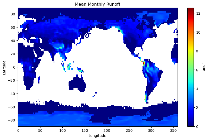
mean_ro.plot(cmap="jet", figsize=(10, 6))
plt.xlabel("Longitude")
plt.ylabel("Latitude")
plt.title("Mean Monthly Runoff")

Text(0.5, 1.0, 'Mean Monthly Runoff')

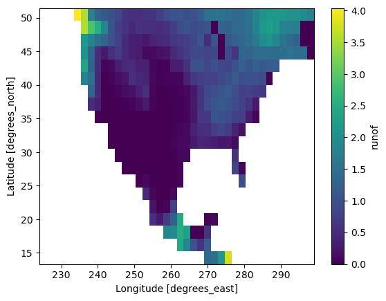
We can use the .isel method to select a spatial subset of the data by index:

cropped_ds = mean_ro.isel(lat=slice(20, 40), lon=slice(120, 160))
cropped_ds.plot()

<matplotlib.collections.QuadMesh at 0x38e70ad50>

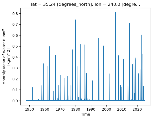
# Plot a time series for a specific location
ro.sel(lat=35.0, lon=240, method="nearest").plot()
plt.show()

GDAL

The Geospatial Data Abstraction Library (GDAL) is the magical piece of open source software that underlies all of the above libraries.

While GDAL has python bindings, the syntax are more complicated and less user friendly than the above libraries. Thus, coverage of GDAL syntax explicitly is outside the scope of this course.

For large batch, big data, or highly custom processing tasks, GDAL has a large array of command-line utilities (see here) that can be deployed via the Anaconda Prompt command line that was introduced in module 1.