4. Python data science modules#
Now that we have a grasp on the fundamentals of Python, we’re ready to use Python for data science.
Unlike some more math-oriented programming languages (like R or MATLAB), Python relies on external packages to provide most data science functionality.
The Python community has standardized on the following family of related packages, all of which we’ll be covering in this module, and will be using extensively for the rest of the course:
numpy - math tools, plus working with 1D & multi-dimensional arrays
pandas - working with tabular data
matplotlib - making plots and visualizations
Numpy#
Numpy is a Python package for representing array data, and comes with a large library of tools and mathematical functions that operate efficiently on arrays, mostly through its ndarray class.
Numpy is by far the most popular Python package for data science, and is one of the most-downloaded python packages overall. It’s so useful and reliable, that most of the mathematical functionality of the other packages covered in this module (pandas, seaborn, matplotlib) is provided by numpy under the hood.
Because numpy is used a lot, it’s convention to import it with the np abbreviation:
import numpy as np
Why numpy?#
A numpy array is similar to a Python list: they can both serve as containers for numbers.
python_list = [0, 2, 4, 6]
print(python_list)
[0, 2, 4, 6]
numpy_array = np.array([0, 2, 4, 6])
print(numpy_array)
[0 2 4 6]
So why use numpy instead of lists?
Speed
Although numpy is a Python package, most of the functionality is written in fast C or Fortran code.
Memory efficient
Numpy uses less memory to store numbers than Python, so you can work on larger datasets.
Functionality
Numpy comes with a huge range of modules with fast and thoroughly-validated algorithms from interpolation to fourier transforms. (We’ll cover many of these functions shortly!)
Manipulation syntax
Numpy’s syntax makes it clear and easy to perform common array operations, like slicing, filtering, and summarization.
But there are some usecases where lists make more sense
Storing different kinds of data together
Numpy arrays are homogeneous, all the elements must be the same type
Working with non-numerical data
Only some numpy functionality works with strings and other types
Creating arrays#
One way to create an array is from a Python sequence like a list using the array() function
days_per_month_list = [31, 28, 31, 30, 31, 30, 31, 31, 30, 31, 30, 31]
days_per_month = np.array(days_per_month_list)
days_per_month
array([31, 28, 31, 30, 31, 30, 31, 31, 30, 31, 30, 31])
Nesting lists will create higher dimensional arrays.
array_2d = np.array([[1, 2, 3, 4], [5, 6, 7, 8], [9, 10, 11, 12]])
array_2d
array([[ 1,  2,  3,  4],
       [ 5,  6,  7,  8],
       [ 9, 10, 11, 12]])
As well as converting Python lists to arrays, numpy can create its own arrays!
You can create an array that’s filled with zeros (helpful for creating an empty array we’ll fill up later)
np.zeros(5)
array([0., 0., 0., 0., 0.])
or ones (for 2D arrays we specify the number of rows, then the number of columns for a 2D array)
np.ones((2, 5))
array([[1., 1., 1., 1., 1.],
       [1., 1., 1., 1., 1.]])
Numpy has it’s own version of the Python range() function:
np.arange(2, 9, 2)
array([2, 4, 6, 8])
and a related linspace() function to create an array with evenly-spaced elements.
np.linspace(0, 10, num=5)
array([ 0. , 2.5, 5. , 7.5, 10. ])
There’s a whole random module that can create arrays from randomly sampling various distributions
np.random.uniform(low=0, high=10, size=(2, 5))
array([[5.5271    , 8.35305849, 6.00420935, 5.18776996, 9.34947434],
       [6.61502902, 0.20982672, 4.53692684, 4.68884583, 9.82653392]])
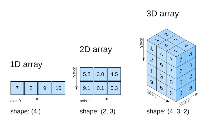
Size and shape#
We can use len() to get the length of a 1D array
len(days_per_month)
12
while the .shape attribute will give the length of each dimension (remember the 2D order? rows then cols!)
array_2d.shape
(3, 4)
Array arithmetic#
Arrays let you express mathematical equations without for loops. This makes your code much faster, plus numpy code tends to read more like a math formula than programming.
Operations with single numbers are applied to the whole array
weeks_per_month = days_per_month / 7
print(weeks_per_month)
[4.42857143 4.         4.42857143 4.28571429 4.42857143 4.28571429
 4.42857143 4.42857143 4.28571429 4.42857143 4.28571429 4.42857143]
whereas operations between arrays of the same size are applied element-wise
days_per_month + days_per_month
array([62, 56, 62, 60, 62, 60, 62, 62, 60, 62, 60, 62])
Comparing arrays results in an array of the same size with True/False values.
days_per_month >= 31
array([ True, False,  True, False,  True, False,  True,  True, False,
        True, False,  True])
To perform element-wise boolean logic between arrays, numpy uses & instead of and, and | instead of or.
(np.arange(12) < 3) & (days_per_month >= 31)
array([ True, False,  True, False, False, False, False, False, False,
       False, False, False])
These boolean arrays can be stored as variables like any other. Creating intermediary variables can make arithmetic logic easier to read
is_long_month = days_per_month >= 31
is_q1_month = np.arange(12) < 3
is_long_q1_month = is_q1_month & is_long_month
print(is_long_q1_month)
[ True False True False False False False False False False False False]
Array slicing and indexing#
Like a Python list, arrays can be sliced
days_per_month[0:3]
array([31, 28, 31])
and individual elements can be index out
print(days_per_month[1])
28
You index a 2D array using the same notation: first your row slicing, then a comma ,, then your column slicing.
Here’s our array as a reminder
array_2d
array([[ 1,  2,  3,  4],
       [ 5,  6,  7,  8],
       [ 9, 10, 11, 12]])
For example, in the 2nd row, and the 1st column
print(array_2d[1, 0])
5
or the first three rows of the last column
print(array_2d[0:3, -1])
[ 4 8 12]
Note how our column has lost its “verticalness”: once we’ve sliced it out, it’s just a regular 1D array.
Assigning new values to an array uses the same slice syntax: arrays are mutable!
A single value will be repeated to all elements (a : without numbers means all elements):
array_2d[0, :] = 99
array_2d
array([[99, 99, 99, 99],
       [ 5,  6,  7,  8],
       [ 9, 10, 11, 12]])
while an equal-length sequence will be assigned elementwise
array_2d[:, 3] = [-1, -2, -3]
array_2d
array([[99, 99, 99, -1],
       [ 5,  6,  7, -2],
       [ 9, 10, 11, -3]])
If we make a slice then modify it, the original array is modified too!
array_2d_slice = array_2d[1:2, 2:3]
array_2d_slice[0] = -9999
array_2d
array([[   99,    99,    99,    -1],
       [    5,     6, -9999,    -2],
       [    9,    10,    11,    -3]])
To keep numpy’s speedy performance, making a slice doesn’t copy any data, just provides a “view” to the original array.
If we want to modify a subset of the data independently, we can use the copy method.
q1_months = days_per_month[:3]
q1_months_leap_year = q1_months.copy()
q1_months_leap_year[1] = 29
q1_months_leap_year
array([31, 29, 31])
Data types#
All values in a numpy array are converted to be the same type. By default, numpy will take an educated guess about what type we want, and we can see its choice with the dtype attribute
array_default = np.array([1, 2, 3])
array_default.dtype
dtype('int64')
We can override the dtype though
array_manual = np.array([1, 2, 3], dtype=np.float64)
array_manual.dtype
dtype('float64')
Other than ints and floats, the boolean dtype is frequently used in numpy
is_positive = array_2d > 0
is_positive.dtype
dtype('bool')
Arrays can store strings, though of course some numpy mathematical tools won’t work
states = np.array(["Washington", "Oregon", "California"])
states.dtype
dtype('<U10')
The U in <U10 stands for “Unicode string”. The < and 10 characters represent internal numpy storage attributes (endianess and number of characters respectively).
An array can also store arbitrary python objects. Lets make an array containing a number as well as the print() function
# This is a terrible idea.
mixed = np.array([42, print])
mixed.dtype
dtype('O')
Numpy gives up and applies the O for “object” dtype (everything in Python is an object).
If you see this in the real world, it’s usually a sign that you’re number parsing has gone wrong! Otherwise, you may as well use a regular list.
Boolean indexing#
Here are some state names, with corresponding mean annual precipitation.
states = np.array(["Washington", "Oregon", "California"])
precip = np.array([38.67, 43.62, 22.97])
To pick out California we can use == to create a boolean array
states == "California"
array([False, False, True])
Passing this boolean array as indexing to another array of the same length will slice out only the elements matching True
precip[states == "California"]
array([22.97])
This is really powerful for working between corresponding arrays!
Negation can be done with !=
precip[states != "California"]
array([38.67, 43.62])
or by using ~ to flip all the booleans in an array
~(states == "California")
array([ True, True, False])
match = states == "California"
precip[~match]
array([38.67, 43.62])
We can also filter the other way
high_rainfall = precip > 30
states[high_rainfall]
array(['Washington', 'Oregon'], dtype='<U10')
Mathematical functions#
Numpy comes with array versions of the functions in the builtin math module, and many more.
Many are element-wise transformations
nums = np.linspace(0, 100, 4)

print(nums)
print(np.floor(nums))  # Round down to next integer.
[  0.          33.33333333  66.66666667 100.        ]
[  0.  33.  66. 100.]
while others summarize
np.median(nums)
np.float64(50.0)
For multidimensional arrays, summarizing functions still give a single overall result
array_2d = np.array([[1, 2, 3, 4], [5, 6, 7, 8], [9, 10, 11, 12]])
np.mean(array_2d)
np.float64(6.5)
But we can specify which dimension the function should summarize using the axis argument. This will be useful later when dealing with observation data that might have at least x, y, and time dimensions.
To get the mean of each row:
np.mean(array_2d, axis=1)
array([ 2.5, 6.5, 10.5])
Here’s a few of the more common numpy functions
Element-wise
sin,arcsine,deg2rad: trigonometryround,floor,ceil: roundingexp,log,log10: logarithmsclip: limit the elements in an array
Summarizing
mean,median,mode: averagesstd,var: skewsum,prod: sum/product of all elementspercentile,quantile: order
Because numpy is so foundational to scientific Python, if you can’t find a common math algorithm in numpy, there’s likely to be another package that provies the function with full support for numpy arrays.
Good places to hunt for extended math functions include
scipy has many submodules including functions for interpolation, statistics, and linear algebra
statsmodels for summary statistics
pandas has functions for dealing with time series and strings
NaNs#
NaN stands for “Not a Number”.
They can come from importing missing data
values = ["1", None, "3"]
np.array(values, dtype=np.float64)
array([ 1., nan, 3.])
or as the result of mathematical operations
# You see a warning message after running this cell!
#
# Numpy can perform mathematical operations on NaN values without errors.
# But often this is a sign that something has gone wrong, so it gives you
# a helpful heads up.
np.arange(5) / np.arange(5)
/var/folders/df/w347rlh96tx42h1kl69_4r8w0000gn/T/ipykernel_45839/2500404429.py:6: RuntimeWarning: invalid value encountered in divide
  np.arange(5) / np.arange(5)
array([nan, 1., 1., 1., 1.])
but most commonly come from other NaNs!
NaNs propagate. The result of an operation where any of the inputs is NaN, usually results in a NaN output, which can spread to your entire dataset!
array_2d = np.array([[np.nan, 2, 3, 4], [5, 6, 7, 8], [9, 10, 11, 12]])
array_2d
array([[nan,  2.,  3.,  4.],
       [ 5.,  6.,  7.,  8.],
       [ 9., 10., 11., 12.]])
array_2d_normalized = array_2d / np.max(array_2d)
array_2d_normalized
array([[nan, nan, nan, nan],
       [nan, nan, nan, nan],
       [nan, nan, nan, nan]])
There are a few things we can do to manage and embrace NaN values.
First, if you can’t discard invalid numerical data, then explicitly convert it to NaN.
flowrate_over_time = np.array([None, 1.9, 2.1, 3.0, -1, 4.3, 4.8], dtype=np.float64)

# Remove invalid data. The sensor returns -1 when broken.
flowrate_over_time[flowrate_over_time < 0] = np.nan

flowrate_over_time
array([nan, 1.9, 2.1, 3. , nan, 4.3, 4.8])
If you want to ignore NaNs, many numpy functions have nan-ignoring siblings.
np.nanmax(array_2d)
np.float64(12.0)
You’ll still get a NaN result if your entire input array is NaN though
np.nanmean(array_2d_normalized)
/var/folders/df/w347rlh96tx42h1kl69_4r8w0000gn/T/ipykernel_45839/2690959602.py:1: RuntimeWarning: Mean of empty slice
  np.nanmean(array_2d_normalized)
np.float64(nan)
If you’re not expecting any NaNs, enforce that in the code. Numpy has some helpful functions for this.
np.isnan() returns a boolean array that is True for NaN values
np.isnan(flowrate_over_time)
array([ True, False, False, False, True, False, False])
np.isfinite() is similar: it will be False for both NaN values as well as Inf (infinity) values
np.isfinite(flowrate_over_time)
array([False, True, True, True, False, True, True])
Numpy also has np.any() and np.all() that will return a single boolean value that is true of any/all of the elements are True
np.all([True, False])
np.False_
np.any([True, False])
np.True_
With all that in mind, a common quick data validation statement might look like
# All days of the month should be real integers!
assert np.all(np.isfinite(days_per_month)), "Invalid data found!"
Exercise: numpy flow#
Let’s generate some synthetic data, filter some outliers, then perform an analysis on the remaining data.
Generate data for the depth (in meters) of 100 different wells.
Build a numpy array containing 100 random numbers between -20 and 20.
You may want to use the numpy random tool.
Negative well depths represent sensor errors.
Set all the negative values to
NaN.
Remove all the
NaNvalues.Print the length of the array before and after the
NaNremoval step, so you can see how your data has changed.
Calculate the median of the remaining values.
Things to think about
What should my variables be called?
Do the results change when you rerun the code?
Extra: What other summary statistics does numpy have that could be interesting to know?
Extra: How can I “seed” the random number generation, so that the numbers are still drawn from a random distribution, but the array will have the same values every time the code is run (for reproducability)?
Extra: What would happen if you got unlucky and all 100 values were negative? How could you modifiy the code to try out this scenario? How could you handle that possibility in code?
Pandas#
Pandas is a package for working with tabular spreadsheet-like data.
What is tabular data?#
Tabular data is anything in a table form!
Common analytical examples include spreadsheets, CSV files, and database tables.
Tabular data consists of rows and columns:
Each row represents an item, and each column represents a common feature of all the items.
Each row has the same columns as the other rows, in the same order.
A single column holds data of the same type, but different columns can have different types.
The order of rows sometimes matters, while the order of columns doesn’t matter.
Tabular data isn’t just work spreadsheets either: for example, a music playlist is tabular data (for each song, we know the title, genre, etc) and your text message inbox is tabular data (for each conversation, we know the participants, unread status, date of most recent message, etc)
Because pandas is so frequently used, it’s standard to import with the pd abbreviation.
import pandas as pd
Loading data#
Pandas comes with many functions for reading lots of different kinds of data. We’ll cover most of them by the end of the course, but here’s a list of the main ones for your later reference
CSVs (read_csv)
SQL databases (read_sql)
Excel files (read_excel)
Parquet files (read_parquet)
Any of the above, as a URL
To start off, we’ll load this CSV file of ground water stations.
url = "https://raw.githubusercontent.com/py4wrds/py4wrds/refs/heads/module-4/data/gwl/stations.csv"
df = pd.read_csv(url)
Note that we’re loading the data directly from GitHub! This won’t work for private repositories, there you’ll have to download the file and use the filepath instead of the url.
DataFrames#
The code above (df = pd.read_csv(url)) has loaded our tabular data into an object called a DataFrame:
type(df)
pandas.core.frame.DataFrame
The DataFrame is one of the two core classes that pandas gives us (the other is Series which represents a column).
DataFrame has a number of attributes (variables) and methods (functions) for inspecting our data, which is the first step in any analysis!
head() shows us the first five rows of data
df.head()
| STN_ID | SITE_CODE | SWN | WELL_NAME | LATITUDE | LONGITUDE | WLM_METHOD | WLM_ACC | BASIN_CODE | BASIN_NAME | COUNTY_NAME | WELL_DEPTH | WELL_USE | WELL_TYPE | WCR_NO | ZIP_CODE | |
|---|---|---|---|---|---|---|---|---|---|---|---|---|---|---|---|---|
| 0 | 51445 | 320000N1140000W001 | NaN | Bay Ridge | 35.5604 | -121.755 | USGS quad | Unknown | NaN | NaN | Monterey | NaN | Residential | Part of a nested/multi-completion well | NaN | 92154 |
| 1 | 25067 | 325450N1171061W001 | 19S02W05K003S | NaN | 32.5450 | -117.106 | Unknown | Unknown | 9-033 | Coastal Plain Of San Diego | San Diego | NaN | Unknown | Unknown | NaN | 92154 |
| 2 | 25068 | 325450N1171061W002 | 19S02W05K004S | NaN | 32.5450 | -117.106 | Unknown | Unknown | 9-033 | Coastal Plain Of San Diego | San Diego | NaN | Unknown | Unknown | NaN | 92154 |
| 3 | 39833 | 325450N1171061W003 | 19S02W05K005S | NaN | 32.5450 | -117.106 | Unknown | Unknown | 9-033 | Coastal Plain Of San Diego | San Diego | NaN | Unknown | Unknown | NaN | 92154 |
| 4 | 25069 | 325450N1171061W004 | 19S02W05K006S | NaN | 32.5450 | -117.106 | Unknown | Unknown | 9-033 | Coastal Plain Of San Diego | San Diego | NaN | Unknown | Unknown | NaN | 92154 |
Because our table has so many columns, not all are visible. We can use the .columns attribute to get all the names on one screen
df.columns
Index(['STN_ID', 'SITE_CODE', 'SWN', 'WELL_NAME', 'LATITUDE', 'LONGITUDE',
       'WLM_METHOD', 'WLM_ACC', 'BASIN_CODE', 'BASIN_NAME', 'COUNTY_NAME',
       'WELL_DEPTH', 'WELL_USE', 'WELL_TYPE', 'WCR_NO', 'ZIP_CODE'],
      dtype='object')
How much data are we working with? .shape gives us both the row and column count, which is always in row, col order
print(df.shape)
(43807, 16)
but it’s more clear to take the length directly:
print("n_rows: {}".format(len(df)))
print("n_cols: {}".format(len(df.columns)))
n_rows: 43807
n_cols: 16
dtypes shows the data type of each column.
This is important to check! Pandas makes some guesses about what data type to use, and often gets things wrong. Common pitfalls to be wary of include
Dates might be loaded as strings instead of rich datetime objects.
Numerical columns like
$145or78%might be loaded as strings instead of as numbersA single row with a typo (
32.111!) or a non-numeric placeholder (usingUnknowninstead ofNaN) will turn an other-wise numeric column into a string type.Pandas defaults to using 64 bit integers and floats. If your dataset is maxing out your memory, you can specify 32 bit (or smaller) dtypes to reduce the size once loaded.
ZIP codes should be parsed as strings not integers, to avoid stripping ZIPs that begin with zero.
print(df.dtypes)
STN_ID           int64
SITE_CODE       object
SWN             object
WELL_NAME       object
LATITUDE       float64
LONGITUDE      float64
WLM_METHOD      object
WLM_ACC         object
BASIN_CODE      object
BASIN_NAME      object
COUNTY_NAME     object
WELL_DEPTH     float64
WELL_USE        object
WELL_TYPE       object
WCR_NO          object
ZIP_CODE         int64
dtype: object
We can see pandas has done a pretty good job here! (the object type is what pandas uses to represent strings).
Fixing some dtype issues can involve more complex analysis. But for simple cases, we can simply tell pandas what to do when loading the data:
df = pd.read_csv(url, dtype={"ZIP_CODE": str})
describe() gives a summary of our numerical columns. With the reloaded dataframe, ZIP_CODE is no longer considered numeric!
df.describe()
| STN_ID | LATITUDE | LONGITUDE | WELL_DEPTH | |
|---|---|---|---|---|
| count | 43807.000000 | 43807.000000 | 43807.000000 | 11646.000000 |
| mean | 25718.430753 | 35.957077 | -119.233081 | 470.534003 |
| std | 14618.354046 | 1.795673 | 1.850751 | 470.431239 |
| min | 2000.000000 | 32.545000 | -124.330000 | 0.000000 |
| 25% | 13455.500000 | 34.610600 | -120.568000 | 148.000000 |
| 50% | 24625.000000 | 35.919700 | -119.413000 | 308.000000 |
| 75% | 35987.500000 | 37.007250 | -117.423000 | 615.000000 |
| max | 55326.000000 | 42.012700 | -114.134000 | 3000.000000 |
Finally, we’re not always interested in the whole dataset for every analysis. You can load a subset of the columns to speed up loading, reduce memory pressure, and to just keep your workspace tidier:
df_county = pd.read_csv(url, usecols=["STN_ID", "WELL_DEPTH"])

df_county.tail()
| STN_ID | WELL_DEPTH | |
|---|---|---|
| 43802 | 37755 | 125.0 |
| 43803 | 25155 | 600.0 |
| 43804 | 38726 | 95.0 |
| 43805 | 26004 | 380.0 |
| 43806 | 26051 | 300.0 |
Based on the output of df_county.tail(), what do you think the tail() method does?
As well as reading DataFrames from files, they can also be constructed using a dict Python sequences. Each column must be the same length (it’s OK to mix lists, arrays, tuples, etc) or be a single value (which will be repeated for the whole column)
df_from_dict = pd.DataFrame(
    {
        "state": ["Washington", "Oregon", "California"],
        "precip": np.array([38.67, 43.62, 22.97]),
        "country": "USA",
    }
)
Series#
A column of a dataframe is a Series object. You can access a column by using its name in [] brackets, just like a dictionary:
type(df["BASIN_NAME"])
pandas.core.series.Series
df["COUNTY_NAME"]
0           Monterey
1          San Diego
2          San Diego
3          San Diego
4          San Diego
            ...
43802    Klamath, OR
43803    Klamath, OR
43804    Klamath, OR
43805    Klamath, OR
43806    Klamath, OR
Name: COUNTY_NAME, Length: 43807, dtype: object
You can also access columns with attribute dot notation like df.COUNTY_NAME.
df.COUNTY_NAME
0           Monterey
1          San Diego
2          San Diego
3          San Diego
4          San Diego
            ...
43802    Klamath, OR
43803    Klamath, OR
43804    Klamath, OR
43805    Klamath, OR
43806    Klamath, OR
Name: COUNTY_NAME, Length: 43807, dtype: object
That’s shorter and clearer! But there are some catches.
The dot notation won’t work when the column name isn’t a valid Python name (like if it contains spaces).
It also won’t work if the column name would override a DataFrame attribute or method (like
head).Finally, you can’t use the dot notation for assignment (the code
df.WELL_DEPTH = np.nanwon’t work).
For those reasons, it can be simpler to just use df["column_name"] syntax always.
We can convert a Series to a list with to_list()
df["COUNTY_NAME"].to_list()[:5]
['Monterey', 'San Diego', 'San Diego', 'San Diego', 'San Diego']
or to a numpy array
df["WELL_DEPTH"].to_numpy()[-5:]
array([125., 600., 95., 380., 300.])
Series supports boolean slicing with []
is_san_diego = df["COUNTY_NAME"] == "San Diego"
san_diego_ids = df["STN_ID"][is_san_diego]

san_diego_ids
1       25067
2       25068
3       39833
4       25069
5       38479
        ...
3142    10637
3181    31281
3183    31280
3195    31295
3400    10634
Name: STN_ID, Length: 2474, dtype: int64
However, to slice by positional integer, you need to use .iloc[] (for integer locaction)
series_head = df["COUNTY_NAME"].iloc[0:5]
series_head
0     Monterey
1    San Diego
2    San Diego
3    San Diego
4    San Diego
Name: COUNTY_NAME, dtype: object
Otherwise a pandas Series is very similar to a numpy array (often a numpy array is being used by pandas to store a Series!). You can do slicing, indexing, arithmetic, and boolean logic just like in numpy.
Series methods#
Pandas columns come with a range of helpful methods.
There are methods for most of the same math equations as numpy: min max, mean mode median quantile, sum, etc. Unlike numpy, pandas methods tend to ignore NaN values.
print(df["WELL_DEPTH"].sum())
5479839.0
There are methods for unique values. If a column is all the same, that could signify a data issue, or perhaps mean we we don’t need to load that column.
assert df["STN_ID"].is_unique, "There should be no duplicated IDs"
assert df["COUNTY_NAME"].nunique() > 1, "Ensure we're not using a single-county subset"
A particularly useful method is value_counts. Used for summarizing discreet value distribution, it displays the count of each unique value.
By default, NaN values aren’t included, but for data exploration it’s really important to know where our NaNs are so we add dropna=False!
df["WELL_USE"].value_counts(dropna=False)
WELL_USE
Unknown          29458
Irrigation        6052
Observation       3910
Residential       1858
NaN               1400
Other              392
Public Supply      391
Stockwatering      208
Industrial         138
Name: count, dtype: int64
If only the unique names are needed without the counts, the unique() method provides that
df["WELL_USE"].unique()
array(['Residential', 'Unknown', 'Observation', 'Other', 'Irrigation',
       'Industrial', 'Public Supply', 'Stockwatering', nan], dtype=object)
Column wrangling#
By passing a list of column names, we can slice all rows for only the specified columns.
(Note the double brackets: one set for the indexing, and another pair for the list):
df[["BASIN_NAME", "COUNTY_NAME"]].head()
| BASIN_NAME | COUNTY_NAME | |
|---|---|---|
| 0 | NaN | Monterey |
| 1 | Coastal Plain Of San Diego | San Diego |
| 2 | Coastal Plain Of San Diego | San Diego |
| 3 | Coastal Plain Of San Diego | San Diego |
| 4 | Coastal Plain Of San Diego | San Diego |
New columns can be added as a singular value
df["country_code"] = "US"
or with any list/Series/array of the same length as the DataFrame (pandas will convert it to a Series)
site_code_prefix = []
for code in df.SITE_CODE:
    if code:
        site_code_prefix.append(code.split("N")[0])
    else:
        site_code_prefix.append(None)

df["site_code_prefix"] = site_code_prefix
or by performing calculations between columns (loc is used for non-integer slicing, like by column name)
df["well_depth_m"] = df.WELL_DEPTH / 3.28084
df[["site_code_prefix", "well_depth_m"]].tail()
| site_code_prefix | well_depth_m | |
|---|---|---|
| 43802 | 419995 | 38.099999 |
| 43803 | 420008 | 182.879994 |
| 43804 | 420050 | 28.955999 |
| 43805 | 420127 | 115.823996 |
| 43806 | 420171 | 91.439997 |
Single columns can be deleted with the del keyword
del df["ZIP_CODE"]

print("ZIP_CODE" in df)
False
and for multiple columns, there’s a drop method.
df = df.drop(columns=["site_code_prefix", "well_depth_m"])

print("site_code_prefix" in df)
False
Filtering and slicing#
We’ve already seen the head() method, which shows the first n rows.
A similar function is the sample() method, which shows n random rows. This can give a better sense of the data, in case the first few rows aren’t representative of the rest.
df.sample(n=7)
| STN_ID | SITE_CODE | SWN | WELL_NAME | LATITUDE | LONGITUDE | WLM_METHOD | WLM_ACC | BASIN_CODE | BASIN_NAME | COUNTY_NAME | WELL_DEPTH | WELL_USE | WELL_TYPE | WCR_NO | country_code | |
|---|---|---|---|---|---|---|---|---|---|---|---|---|---|---|---|---|
| 31855 | 32837 | 369071N1207449W001 | 12S11E11D003M | NaN | 36.9071 | -120.745 | Unknown | Unknown | 5-022.07 | Delta-Mendota | Fresno | NaN | Unknown | Unknown | NaN | US |
| 32937 | 52350 | 370148N1215633W001 | 10S04E32N003M | 10S04E32N003 | 37.0148 | -121.563 | Surveyed | 0.1 ft. | 3-003.01 | Llagas Area | Santa Clara | 0.0 | Observation | Single Well | NaN | US |
| 42179 | 33574 | 395892N1217304W001 | 20N02E15H002M | BMO 20N02E15H002M | 39.5892 | -121.730 | Surveyed to a benchmark | 0.1 ft. | 5-021.70 | Butte | Butte | 75.0 | Observation | Single Well | 454084 | US |
| 1158 | 31846 | 332317N1169887W001 | 11S01W09K002S | NaN | 33.2317 | -116.989 | Unknown | Unknown | NaN | NaN | San Diego | NaN | Unknown | Unknown | NaN | US |
| 20595 | 21764 | 356975N1173662W001 | 26S43E04N001M | NaN | 35.6975 | -117.366 | Unknown | Unknown | 6-052 | Searles Valley | San Bernardino | NaN | Unknown | Unknown | NaN | US |
| 18557 | 35244 | 353855N1153291W001 | 15N15E13G001S | NaN | 35.3855 | -115.329 | Unknown | Unknown | 6-030 | Ivanpah Valley | San Bernardino | NaN | Unknown | Unknown | NaN | US |
| 28385 | 25740 | 366034N1203701W002 | 15S15E20N008M | NaN | 36.6034 | -120.370 | Unknown | Unknown | 5-022.09 | Westside | Fresno | NaN | NaN | Unknown | NaN | US |
Technically what we’re doing here isn’t just printing some rows of our dataset, but actually creating a new DataFrame with some rows sliced from the old one, and printing that new frame.
There are some other DataFrame methods that return a new dataframe with a subset of rows. drop_duplicates() returns a DataFrame with repeated rows removed. dropna returns a dataframe with only rows that don’t have any NaN values:
df_unique = df.drop_duplicates()
df_clean = df_unique.dropna()
len(df_clean)
4027
Because these are both DataFrame methods that return another DataFrame, we can chain them together to save space
df_clean = df.drop_duplicates().dropna()
len(df_clean)
4027
Most pandas methods return a new DataFrame rather than modifying the original one. We can see that our original still has the same number of rows:
len(df)
43807
.iloc does integer indexing on a DataFrame too, but it’s clearer to use the column names rather than their positional index. For that, .loc allows us to filter by both row and col at once (remember the row, col order).
# Get all the USGS rows, and keep only the positional data.
df_USGS = df.loc[df.WCR_NO == "USGS", ["WCR_NO", "LATITUDE", "LONGITUDE"]]
df_USGS.head()
| WCR_NO | LATITUDE | LONGITUDE | |
|---|---|---|---|
| 39035 | USGS | 38.3759 | -121.955 |
| 39891 | USGS | 38.6313 | -121.894 |
| 40978 | USGS | 38.9552 | -122.097 |
| 41118 | USGS | 38.9884 | -122.007 |
| 41299 | USGS | 39.0429 | -122.054 |
.loc is also used in pandas for assignment of a subset of rows/cols.
# For every row with COUNTY_NAME equal to "Monterey", set that row's WELL_USE value to Residential.
df.loc[df.COUNTY_NAME == "Monterey", "WELL_USE"] = "Residential"
df.head()
| STN_ID | SITE_CODE | SWN | WELL_NAME | LATITUDE | LONGITUDE | WLM_METHOD | WLM_ACC | BASIN_CODE | BASIN_NAME | COUNTY_NAME | WELL_DEPTH | WELL_USE | WELL_TYPE | WCR_NO | country_code | |
|---|---|---|---|---|---|---|---|---|---|---|---|---|---|---|---|---|
| 0 | 51445 | 320000N1140000W001 | NaN | Bay Ridge | 35.5604 | -121.755 | USGS quad | Unknown | NaN | NaN | Monterey | NaN | Residential | Part of a nested/multi-completion well | NaN | US |
| 1 | 25067 | 325450N1171061W001 | 19S02W05K003S | NaN | 32.5450 | -117.106 | Unknown | Unknown | 9-033 | Coastal Plain Of San Diego | San Diego | NaN | Unknown | Unknown | NaN | US |
| 2 | 25068 | 325450N1171061W002 | 19S02W05K004S | NaN | 32.5450 | -117.106 | Unknown | Unknown | 9-033 | Coastal Plain Of San Diego | San Diego | NaN | Unknown | Unknown | NaN | US |
| 3 | 39833 | 325450N1171061W003 | 19S02W05K005S | NaN | 32.5450 | -117.106 | Unknown | Unknown | 9-033 | Coastal Plain Of San Diego | San Diego | NaN | Unknown | Unknown | NaN | US |
| 4 | 25069 | 325450N1171061W004 | 19S02W05K006S | NaN | 32.5450 | -117.106 | Unknown | Unknown | 9-033 | Coastal Plain Of San Diego | San Diego | NaN | Unknown | Unknown | NaN | US |
Looping over DataFrames#
To loop over a single column (Series) you can use it directly in a standard for loop:
for county in df.head()["COUNTY_NAME"]:
    print(county)
Monterey
San Diego
San Diego
San Diego
San Diego
To loop over a few columns at a time, you can use Python’s builtin zip function:
for stn_id, county in zip(df.head()["STN_ID"], df.head()["COUNTY_NAME"]):
    print("{}, {}".format(stn_id, county))
51445, Monterey
25067, San Diego
25068, San Diego
39833, San Diego
25069, San Diego
To loop over each row at a time, the most robust approach is to convert the DataFrame to a list of dicts. (You must use the orient="records" argument as there are many other ways to format the data as a dictionary)
for row_dict in df.head().to_dict(orient="records"):
    print("{}, {}".format(row_dict["STN_ID"], row_dict["COUNTY_NAME"]))
51445, Monterey
25067, San Diego
25068, San Diego
39833, San Diego
25069, San Diego
Pandas also has the function itertuples which can sometimes be useful for looping over rows, but it has some tricky blindspots (it doesn’t work for column names with spaces). Note that iteritems was removed in pandas 2.0. Because of these limitations, we recommend using one of the methods mentioned above.
Pandas index#
In the examples above, you might have noticed that when printing a DataFrame or a Series, it also shows a row number.
df.iloc[[1000, 2000, 3000, 4000]][["STN_ID", "BASIN_NAME"]]
| STN_ID | BASIN_NAME | |
|---|---|---|
| 1000 | 32211 | NaN |
| 2000 | 11760 | Lower San Luis Rey Valley |
| 3000 | 12002 | Temecula Valley |
| 4000 | 9362 | Cahuilla Valley |
Every DataFrame and Series has a row ID, which pandas calls an index.
By default the index is the row number, but we could use the actual ID from our dataset for example
df_index = df.set_index(df.STN_ID.to_numpy())
df_index.iloc[[1000, 2000, 3000, 4000]][["STN_ID", "BASIN_NAME"]]
| STN_ID | BASIN_NAME | |
|---|---|---|
| 32211 | 32211 | NaN |
| 11760 | 11760 | Lower San Luis Rey Valley |
| 12002 | 12002 | Temecula Valley |
| 9362 | 9362 | Cahuilla Valley |
Indexes provide very fast lookups of individual rows using the .loc attribute
df_index.loc[12002]
STN_ID                       12002
SITE_CODE       334439N1170645W001
SWN                  08S02W35D001S
WELL_NAME                      NaN
LATITUDE                   33.4439
LONGITUDE                 -117.065
WLM_METHOD                 Unknown
WLM_ACC                    Unknown
BASIN_CODE                   9-005
BASIN_NAME         Temecula Valley
COUNTY_NAME              Riverside
WELL_DEPTH                     NaN
WELL_USE                   Unknown
WELL_TYPE                  Unknown
WCR_NO                         NaN
country_code                    US
Name: 12002, dtype: object
However, it’s rare to access individual rows in analytical applications, so for simplicity we won’t be using indexes in this course.
You can always achieve the same result using boolean indexing
df[df.STN_ID == 12002].iloc[0] # Filter and take the first match.
STN_ID                       12002
SITE_CODE       334439N1170645W001
SWN                  08S02W35D001S
WELL_NAME                      NaN
LATITUDE                   33.4439
LONGITUDE                 -117.065
WLM_METHOD                 Unknown
WLM_ACC                    Unknown
BASIN_CODE                   9-005
BASIN_NAME         Temecula Valley
COUNTY_NAME              Riverside
WELL_DEPTH                     NaN
WELL_USE                   Unknown
WELL_TYPE                  Unknown
WCR_NO                         NaN
country_code                    US
Name: 3000, dtype: object
String series#
As well as numerical data, pandas Series class has methods for working with strings as well.
We’ll demo this with a dataset that has a few more strings: CIWQS NPDES Permits.
df_npdes = pd.read_excel("./data/npdes_data.xlsx", nrows=1000, dtype={"ZIP CODE": str})
df_npdes.head()
| DISCHARGER | DISCHARGER ID | RM STATUS | REGION CODE | REG MEAS ID | ORDER NUMBER | NPDES NUMBER | REG MEAS TYPE | FACILIITY NAME | FACILITY PLACE ID | ... | EXPIRATION DATE | TERMINAITON DATE | STREET ADDRESS | FACILITY CITY | ZIP CODE | COUNTY | DISCHARGER STREET ADDRESS | DISCHARGER CITY | DISCHARGER STATE | DISCHARGER ZIP CODE | |
|---|---|---|---|---|---|---|---|---|---|---|---|---|---|---|---|---|---|---|---|---|---|
| 0 | AC Products Inc | 623 | Active | 8 | 206294 | R8-2012-0027 | CAG918001 | Enrollee | GW Cleanup-Anaheim-AC Product P-2 | 228176.0 | ... | 07/01/2017 | NaN | 1601 Placentia | Anaheim | 92806 | Orange | 9930 Painter Avenue | Whittier | CA | 90605 |
| 1 | Action Motorsports of Tahoe | 732 | Active | 6A | 379813 | R6T-2016-0038 | NaN | Enrollee | Timber Cove Marina | 264519.0 | ... | 11/01/2026 | NaN | 3411 Lake Tahoe Boulevard | South Lake Tahoe | 96157 | El Dorado | Po Box 13356 | South Lake Tahoe | CA | 96151 |
| 2 | Aerojet Rocketdyne, Inc. | 854 | Active | 5S | 441580 | R5-2020-0051 | CA0083861 | NPDES Permits | Aerojet Interim GW Extraction & Treatment System | 232546.0 | ... | 10/31/2025 | NaN | Aerojet Road | Sacramento | 95813-6000 | Sacramento | Po Box 13222 | Sacramento | CA | 95813 |
| 3 | AES Alamitos LLC | 864 | Active | 4 | 437188 | R4-2020-0134 | CA0001139 | NPDES Permits | Alamitos Generating Station | 207266.0 | ... | 12/31/2025 | NaN | 690 North Studebaker Road | Long Beach | 90803 | Los Angeles | 690 North Studebaker Road | Long Beach | CA | 90803 |
| 4 | AES Huntington Beach LLC | 866 | Active | 8 | 422464 | R8-2020-0040 | CA0001163 | NPDES Permits | Huntington Beach Generating Station | 226995.0 | ... | 12/31/2025 | NaN | 21730 Newland Street | Huntington Beach | 92646 | Orange | 21730 Newland Way | Huntington Beach | CA | 92646 |
5 rows × 24 columns
Say we want to pull out all the permits related to AT&T.
The problem is that there’s inconsistent naming of the facilities (this is often the case with user-entered data)
df_npdes.iloc[27:38]["FACILIITY NAME"]
27                          AT&T Statewide Cable System
28    Region 3 - Pacific Bell (a.k.a. SBC) Regionwid...
29    Region 3 - At&T Regionwide Utility Vaults (NPDES)
30                        AT&T Utility Vault Discharges
31                                   AT&T Utility Vault
32                          AT & T/Statewide Utility GP
33                                     At&T Corporation
34                AT&T Utility Vaults in SFBay Region 2
35    AT&T Facilities Under the General Utilities Pe...
36                                Atwater Regional WWTF
37    Atwater WWTF Mun WW Disch that Meet Obj/Criter...
Name: FACILIITY NAME, dtype: object
To address this, lets tidy up the name field. We’ll do this in a new column so we don’t loose our original data.
df_npdes["tidy_name"] = df_npdes["FACILIITY NAME"].copy()
Most of python’s builtin string functions have equivalent pandas Series methods. The pandas methods are much faster though, and for advanced users, many can be used with regular expressions.
# Replace numeric NaN values with empty strings.
df_npdes["tidy_name"] = df_npdes["tidy_name"].fillna("")

# Remove leading/trailing whitespace.
df_npdes["tidy_name"] = df_npdes["tidy_name"].str.strip()

# Convert to uppercase.
df_npdes["tidy_name"] = df_npdes["tidy_name"].str.upper()

# Fix spacing.
df_npdes["tidy_name"] = df_npdes["tidy_name"].str.replace("AT & T", "AT&T")
The new tidy_name column can now be used for filtering. Here we use a boolean index (based on the str.contains() method) to get only the AT&T rows:
df_att = df_npdes[df_npdes["tidy_name"].str.contains("AT&T")]

df_att[["FACILIITY NAME", "tidy_name"]]
| FACILIITY NAME | tidy_name | |
|---|---|---|
| 25 | AT&T Utility vaults | AT&T UTILITY VAULTS |
| 27 | AT&T Statewide Cable System | AT&T STATEWIDE CABLE SYSTEM |
| 29 | Region 3 - At&T Regionwide Utility Vaults (NPDES) | REGION 3 - AT&T REGIONWIDE UTILITY VAULTS (NPDES) |
| 30 | AT&T Utility Vault Discharges | AT&T UTILITY VAULT DISCHARGES |
| 31 | AT&T Utility Vault | AT&T UTILITY VAULT |
| 32 | AT & T/Statewide Utility GP | AT&T/STATEWIDE UTILITY GP |
| 33 | At&T Corporation | AT&T CORPORATION |
| 34 | AT&T Utility Vaults in SFBay Region 2 | AT&T UTILITY VAULTS IN SFBAY REGION 2 |
| 35 | AT&T Facilities Under the General Utilities Pe... | AT&T FACILITIES UNDER THE GENERAL UTILITIES PE... |
| 781 | Pacific Bell (AT&T) | PACIFIC BELL (AT&T) |
We can also normalize to 5-digit zip codes by splitting on the dash, then taking the first group using the str[] indexing tool pandas provides:
df_npdes["tidy_zip_code"] = df_npdes["ZIP CODE"].str.split("-").str[0]

df_npdes[["ZIP CODE", "tidy_zip_code"]].head()
| ZIP CODE | tidy_zip_code | |
|---|---|---|
| 0 | 92806 | 92806 |
| 1 | 96157 | 96157 |
| 2 | 95813-6000 | 95813 |
| 3 | 90803 | 90803 |
| 4 | 92646 | 92646 |
The pandas documentation has a Working with text data guide that goes into more details about regular expressions as well as splitting/joining strings, and has a list of all the string methods.
Timeseries data#
Just like pandas groups string functions with a .str prefix, there is also a .dt prefix that contains functions for working with dates, times, and datetimes (timestamps).
Let’s have a look at some of our date columns:
date_cols = ["ADOPTION DATE", "EFFECTIVE DATE", "EXPIRATION DATE"]
df_npdes[date_cols].head()
| ADOPTION DATE | EFFECTIVE DATE | EXPIRATION DATE | |
|---|---|---|---|
| 0 | NaN | 09/23/2002 | 07/01/2017 |
| 1 | 11/01/2016 | 11/01/2016 | 11/01/2026 |
| 2 | 10/16/2020 | 11/01/2020 | 10/31/2025 |
| 3 | 11/12/2020 | 01/01/2021 | 12/31/2025 |
| 4 | 12/04/2020 | 01/01/2021 | 12/31/2025 |
df_npdes[date_cols].dtypes
ADOPTION DATE      object
EFFECTIVE DATE     object
EXPIRATION DATE    object
dtype: object
The object dtype indicates our dates weren’t parsed correctly. There’s also a numeric NaN mixed in there.
To fix this we’re going to have to go back to the data loading. In this case it’s enough to tell python which columns to treat as dates with the parse_dates argument.
df_npdes = pd.read_excel("./data/npdes_data.xlsx", nrows=1000, parse_dates=date_cols)
df_npdes[date_cols].head()
| ADOPTION DATE | EFFECTIVE DATE | EXPIRATION DATE | |
|---|---|---|---|
| 0 | NaT | 2002-09-23 | 2017-07-01 |
| 1 | 2016-11-01 | 2016-11-01 | 2026-11-01 |
| 2 | 2020-10-16 | 2020-11-01 | 2025-10-31 |
| 3 | 2020-11-12 | 2021-01-01 | 2025-12-31 |
| 4 | 2020-12-04 | 2021-01-01 | 2025-12-31 |
df_npdes[date_cols].dtypes
ADOPTION DATE      datetime64[ns]
EFFECTIVE DATE     datetime64[ns]
EXPIRATION DATE    datetime64[ns]
dtype: object
Now that our dates have the correct type, we can use pandas date/time functionality! Missing/invalid timestamps are specified with NaT (not a timestamp).
For more complex cases, you can use the pd.to_datetime function.
# Convert dates from a dd/mm/yyyy string, halting with an error in the case of any failed conversion.
df["ADOPTION DATE"] = pd.to_datetime(df["ADOPTION DATE"], format="%d/%m/%Y", errors="raise")
The .dt prefix has functions for accessing different parts of the timestamp
# English day of week name. Then replace any None or NaNs with an empty string.
df_npdes["ADOPTION DATE"].dt.day_name().fillna("")
0
1        Tuesday
2         Friday
3       Thursday
4         Friday
         ...
995    Wednesday
996    Wednesday
997       Friday
998    Wednesday
999
Name: ADOPTION DATE, Length: 1000, dtype: object
as well as functions for manipulating timestamps
# Round to the nearest hour (looks like our data is already rounded!).
df_npdes["ADOPTION DATE"].dt.round("h")
0            NaT
1     2016-11-01
2     2020-10-16
3     2020-11-12
4     2020-12-04
         ...
995   2012-12-12
996   2018-08-08
997   2019-03-08
998   2023-11-08
999          NaT
Name: ADOPTION DATE, Length: 1000, dtype: datetime64[ns]
In addition to timestamps, pandas also has the concept of differences between two timestamps.
A Timedelta is a fixed difference:
# Shift dates 7 days forward into the future).
df_npdes["ADOPTION DATE"] + pd.Timedelta(days=7)
0            NaT
1     2016-11-08
2     2020-10-23
3     2020-11-19
4     2020-12-11
         ...
995   2012-12-19
996   2018-08-15
997   2019-03-15
998   2023-11-15
999          NaT
Name: ADOPTION DATE, Length: 1000, dtype: datetime64[ns]
while an offset can vary on length depending on context.
# 10 working days later.
df_npdes["ADOPTION DATE"] + pd.offsets.BusinessDay(n=10)
0            NaT
1     2016-11-15
2     2020-10-30
3     2020-11-26
4     2020-12-18
         ...
995   2012-12-26
996   2018-08-22
997   2019-03-22
998   2023-11-22
999          NaT
Name: ADOPTION DATE, Length: 1000, dtype: datetime64[ns]
Series mapping#
Series has a map() method that applies a regular python function separately to every element.
This is helpful if your function is too complicated to represent using numpy/pandas arithmetic/methods, or if you’d like to use an existing function that doesn’t support arrays.
def tidy_zip_code(code):
    """Normalize and validate zip codes."""
    # Normalize to string.
    if code is None or pd.isna(code):
        return ""
    code = str(code)

    # Normalize to 5 digits.
    code = code.split("-")[0]
    if len(code) == 4:
        code = "0" + code

    # Validate.
    assert len(code) == 5, f"Wrong zip length {code=}"
    return code


df_npdes["validated_zip"] = df_npdes["ZIP CODE"].map(tidy_zip_code)

df_npdes[["ZIP CODE", "validated_zip"]].tail()
| ZIP CODE | validated_zip | |
|---|---|---|
| 995 | 94941 | 94941 |
| 996 | 94941 | 94941 |
| 997 | 94941 | 94941 |
| 998 | 94941 | 94941 |
| 999 | 93263 | 93263 |
The map() method also accepts a dictionary for more simple cases of input -> output mapping
program_descriptions = {
    "INDSTW": "Industrial Stormwater",
    "NPDMINING": "National Pollutant Discharge  - Mining",
    "NPDNONMUNIPRCS": "National Pollutant Discharge  - Non-Municipal - Permit-required Confined Space",
    "NPDMUNILRG": "National Pollutant Discharge  - Large Municipal",
}
df_npdes["full_program_name"] = df_npdes.PROGRAM.map(program_descriptions)

df_npdes[["DISCHARGER", "PROGRAM", "full_program_name"]].head()
| DISCHARGER | PROGRAM | full_program_name | |
|---|---|---|---|
| 0 | AC Products Inc | NPDNONMUNIPRCS | National Pollutant Discharge - Non-Municipal ... |
| 1 | Action Motorsports of Tahoe | INDSTW | Industrial Stormwater |
| 2 | Aerojet Rocketdyne, Inc. | NPDNONMUNIPRCS | National Pollutant Discharge - Non-Municipal ... |
| 3 | AES Alamitos LLC | NPDINDLRG | NaN |
| 4 | AES Huntington Beach LLC | NPDNONMUNIPRCS | National Pollutant Discharge - Non-Municipal ... |
Concatenating and joining DataFrames#
To stack multiple DataFrames that have the same columns, pandas has the concat function.
df_placer = pd.read_csv("data/gwl/Placer.csv")
df_sacramento = pd.read_csv("data/gwl/Sacramento.csv")

df_all = pd.concat([df_placer, df_sacramento])

print(f"{df_placer.shape=}")
print(f"{df_sacramento.shape=}")
print(f"{df_all.shape=}")
df_placer.shape=(184, 14)
df_sacramento.shape=(494, 14)
df_all.shape=(678, 14)
concat stacks rows together by default. But with the axis="columns" argument, we can merge columns from different datasets with the same rows.
df_location = df_placer[["LATITUDE", "LONGITUDE"]]
df_basin = df_placer[["BASIN_CODE", "BASIN_NAME"]]

pd.concat([df_basin, df_location], axis="columns")
| BASIN_CODE | BASIN_NAME | LATITUDE | LONGITUDE | |
|---|---|---|---|---|
| 0 | 5-021.64 | North American | 38.7626 | -121.365 |
| 1 | 5-021.64 | North American | 38.7005 | -121.614 |
| 2 | 5-021.64 | North American | 38.7005 | -121.614 |
| 3 | 5-021.64 | North American | 38.7216 | -121.247 |
| 4 | 5-021.64 | North American | 38.7222 | -121.292 |
| ... | ... | ... | ... | ... |
| 179 | 6-108 | Olympic Valley | 39.1980 | -120.230 |
| 180 | 6-108 | Olympic Valley | 39.1980 | -120.230 |
| 181 | 6-067 | Martis Valley | 39.3006 | -120.112 |
| 182 | 6-067 | Martis Valley | 39.3072 | -120.132 |
| 183 | NaN | NaN | 39.3079 | -120.245 |
184 rows × 4 columns
For more complex database-style joins, we have the pandas.merge function.
Joins combine DataFrames by linking rows based on matching column values.
Lets start by making a DataFrame from a dict of sequences
df_program = pd.DataFrame(
    {
        "PROGRAM": ["INDSTW", "NPDMINING", "NPDNONMUNIPRCS", "NPDMUNILRG"],
        "program_name": [
            "Industrial Stormwater",
            "National Pollutant Discharge  - Mining",
            "National Pollutant Discharge  - Non-Municipal - Permit-required Confined Space",
            "National Pollutant Discharge  - Large Municipal",
        ],
        "program_launch_date": pd.to_datetime(["2024-01-01", "2023-12-20", "2016-01-20", "2024-01-01"]),
    }
)

df_program
| PROGRAM | program_name | program_launch_date | |
|---|---|---|---|
| 0 | INDSTW | Industrial Stormwater | 2024-01-01 |
| 1 | NPDMINING | National Pollutant Discharge - Mining | 2023-12-20 |
| 2 | NPDNONMUNIPRCS | National Pollutant Discharge - Non-Municipal ... | 2016-01-20 |
| 3 | NPDMUNILRG | National Pollutant Discharge - Large Municipal | 2024-01-01 |
and perform a join on the “PROGRAM” column.
# A simple inner join.
df_joined = pd.merge(df_npdes, df_program, on="PROGRAM")

df_joined[["DISCHARGER", "PROGRAM", "program_name", "program_launch_date"]].tail()
| DISCHARGER | PROGRAM | program_name | program_launch_date | |
|---|---|---|---|---|
| 814 | Sewerage Agency of Southern Marin | NPDMUNILRG | National Pollutant Discharge - Large Municipal | 2024-01-01 |
| 815 | Sewerage Agency of Southern Marin | NPDMUNILRG | National Pollutant Discharge - Large Municipal | 2024-01-01 |
| 816 | Sewerage Agency of Southern Marin | NPDMUNILRG | National Pollutant Discharge - Large Municipal | 2024-01-01 |
| 817 | Sewerage Agency of Southern Marin | NPDMUNILRG | National Pollutant Discharge - Large Municipal | 2024-01-01 |
| 818 | Shafter City | NPDNONMUNIPRCS | National Pollutant Discharge - Non-Municipal ... | 2016-01-20 |
Our joined DataFrame has all the columns from both input DataFrames!
You might have noticed that the while df_npdes started off with 1000 rows, the last row number on df_joined is 818!
By default, merge() does an inner merge, which means any rows with a value for PROGRAM that isn’t in both DataFrames is discarded.
Sometimes we do only care about the intersection of two datasets, in which case an inner merge is perfect! But more often in analysis we want to keep our main DataFrame intact, and just enhance with more columns wherever we have data. This is a left join.

Fig. 1 Source: Pratik Joshi#
There’s a couple more tweaks we can make to our join for improved resilience.
Often the joining column will have different names between our dataset. We can specify this with the
left_onandright_onarguments.If our incoming DataFrame has multiple rows with the same join column value, we can end up with extra data post-join. Passing
validate="many_to_one"enforces the lookup style of join.
Here’s a more typical left join:
# A typical data science left join.
df_joined = pd.merge(
    df_npdes,  # Left dataframe
    df_program,  # Right dataframe,
    how="left",
    left_on="PROGRAM",
    right_on="PROGRAM",
    validate="many_to_one",
)


df_joined[["DISCHARGER", "PROGRAM", "program_name", "program_launch_date"]].tail()
| DISCHARGER | PROGRAM | program_name | program_launch_date | |
|---|---|---|---|---|
| 995 | Sewerage Agency of Southern Marin | NPDMUNILRG | National Pollutant Discharge - Large Municipal | 2024-01-01 |
| 996 | Sewerage Agency of Southern Marin | NPDMUNILRG | National Pollutant Discharge - Large Municipal | 2024-01-01 |
| 997 | Sewerage Agency of Southern Marin | NPDMUNILRG | National Pollutant Discharge - Large Municipal | 2024-01-01 |
| 998 | Sewerage Agency of Southern Marin | NPDMUNILRG | National Pollutant Discharge - Large Municipal | 2024-01-01 |
| 999 | Shafter City | NPDNONMUNIPRCS | National Pollutant Discharge - Non-Municipal ... | 2016-01-20 |
Now all 1000 rows are there, and we can clearly identify the added columns.
The pandas documentation has a join guide that goes into more detail about the different join types, validation options, and merge arguments.
Grouping#
Grouping is another operation that will be familiar to those who have worked with databases.
The idea is to categorise rows of a DataFrame into groups, then calculate summary statistics for each group.
You first create a group by passing one or more columns to groupby(). Then define each aggregate with three pieces of information
the name of the result column is the name of the input argument
the first value of the tuple is the group’s column to use
the second value of the tuple is the function to apply to the group. It can be the name of a pandas function as a string, or an actual function.
def active_frac(group):
    """The fraction of the group that has the value 'Active'"""
    return np.mean(group == "Active")


df_npdes.groupby(["DISCHARGER STATE"]).agg(
    n_permits=("DISCHARGER ID", "size"),
    first_adoption=("ADOPTION DATE", np.min),
    active_frac=("RM STATUS", active_frac),
)
/var/folders/df/w347rlh96tx42h1kl69_4r8w0000gn/T/ipykernel_45839/81745869.py:6: FutureWarning: The provided callable <function min at 0x1121f3880> is currently using SeriesGroupBy.min. In a future version of pandas, the provided callable will be used directly. To keep current behavior pass the string "min" instead.
  df_npdes.groupby(["DISCHARGER STATE"]).agg(
| n_permits | first_adoption | active_frac | |
|---|---|---|---|
| DISCHARGER STATE | |||
| CA | 950 | 1990-05-11 | 0.851579 |
| CO | 11 | 2015-08-13 | 1.000000 |
| IL | 1 | NaT | 0.000000 |
| KS | 1 | NaT | 1.000000 |
| MI | 1 | NaT | 1.000000 |
| MN | 1 | NaT | 0.000000 |
| Multiple Addresses | 8 | 2012-12-12 | 0.875000 |
| NJ | 8 | 2006-07-19 | 1.000000 |
| NV | 3 | 2014-07-16 | 0.666667 |
| PA | 2 | NaT | 1.000000 |
| TX | 3 | NaT | 1.000000 |
| VA | 1 | 2012-02-08 | 1.000000 |
| WA | 1 | NaT | 1.000000 |
Plotting with matplotlib#
Because the module name is extremely long, it’s customary to import using
import matplotlib.pyplot as plt
To begin, we’ll load in this DataFrame of groundwater measurements at a 10 different stations over time
df_10 = pd.read_csv("data/gwl/10-sites.csv", usecols=["SITE_CODE", "MSMT_DATE", "GSE_WSE", "COUNTY_NAME"], parse_dates=["MSMT_DATE"])
assert df_10.SITE_CODE.nunique() == 10

df_10.sample(5)
| SITE_CODE | MSMT_DATE | GSE_WSE | COUNTY_NAME | |
|---|---|---|---|---|
| 2608 | 387511N1213389W001 | 1963-08-28 | 106.40 | Placer |
| 2675 | 388974N1213665W001 | 2004-08-04 | 67.80 | Placer |
| 4971 | 384121N1212102W001 | 2018-03-25 | 156.24 | Sacramento |
| 1729 | 386016N1213761W001 | 1999-09-08 | 105.10 | Sacramento |
| 1265 | 385567N1214751W001 | 1999-12-10 | 23.70 | Sacramento |
We start with an empty plot using the subplots() function. This returns two things
a Figure object, which has methods for adjusting the plot layout and saving your plot
one or more Axes objects, which have methods for plotting data
To plot a simple line for a single site, we need the Axes.plot() method, and pass first an array of our x-axis data, then our y-axis data.
df_site = df_10[df_10.SITE_CODE == "384121N1212102W001"]

fig, ax = plt.subplots()
ax.plot(df_site.MSMT_DATE, df_site.GSE_WSE)
[<matplotlib.lines.Line2D at 0x15dd5fed0>]
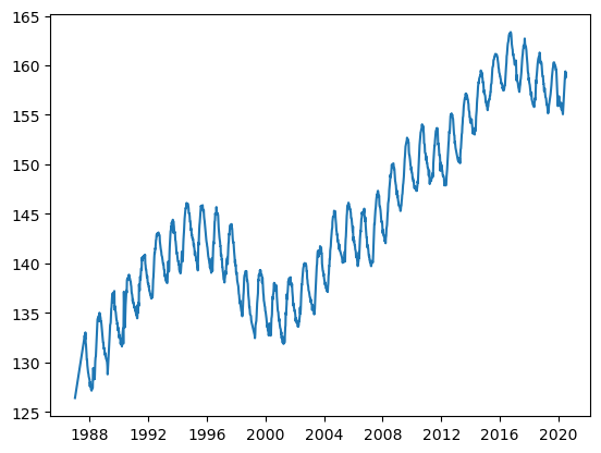
It’s a basic plot but it works!
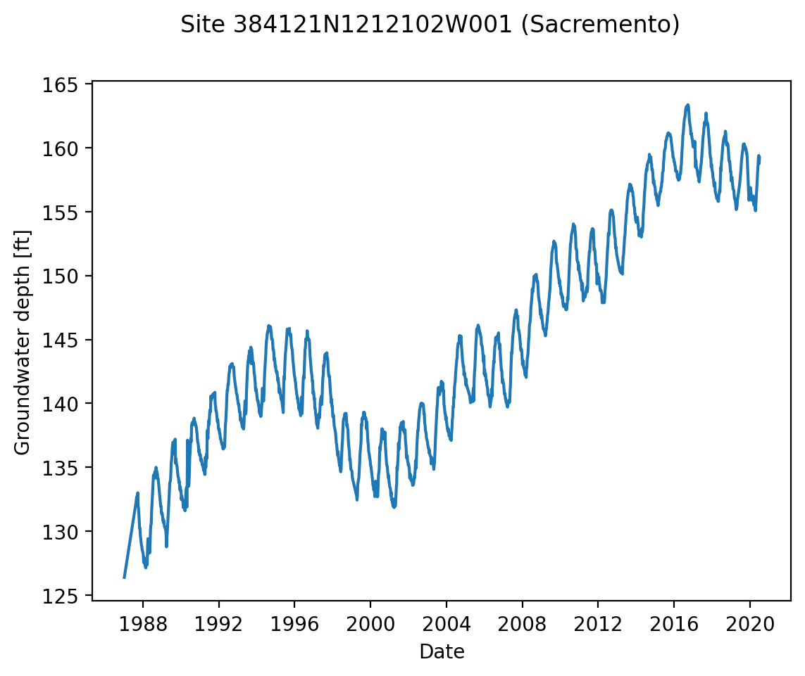
Let’s improve the readability of this plot a bit. Can you see in the code below where each of these changes was made?
Increase the resolution of the image (the default 100 dpi)
Label each axis
Label the entire figure
fig, ax = plt.subplots(dpi=200)
ax.plot(df_site.MSMT_DATE, df_site.GSE_WSE)
ax.set_xlabel("Date")
ax.set_ylabel("Groundwater depth [ft]")
fig.suptitle("Site 384121N1212102W001 (Sacremento)")
Text(0.5, 0.98, 'Site 384121N1212102W001 (Sacremento)')
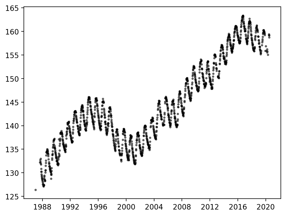
We can visualize the same data using a scatter plot. To show the density of overlapping points, add an alpha keyword where 1 is fully opaque and 0 is fully transparent
fig, ax = plt.subplots(dpi=200)
ax.scatter(
    df_site.MSMT_DATE,
    df_site.GSE_WSE,
    alpha=0.5,  # Each marker is 50% transparent.
    color="black",
    s=5,  # Marker size.
)
<matplotlib.collections.PathCollection at 0x15dd6bcb0>
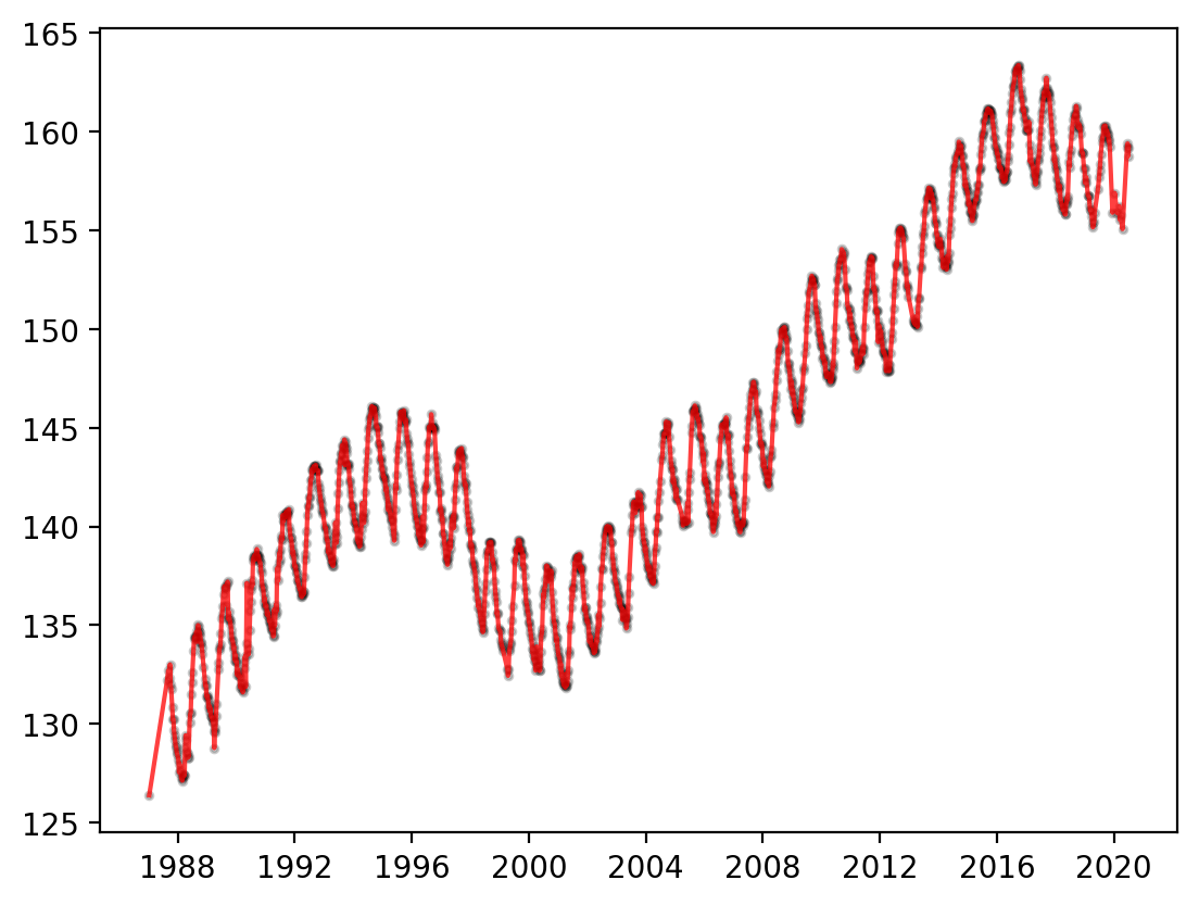
Multiple things can be plotted on the same Axes object. For example, it can be helpful to have both the interpolated line from plot() as well as the observation locations from scatter(). The most recent plot will be on top.
fig, ax = plt.subplots(dpi=200)
ax.scatter(
    df_site.MSMT_DATE,
    df_site.GSE_WSE,
    alpha=0.2,
    color="black",
    s=6,
)
ax.plot(df_site.MSMT_DATE, df_site.GSE_WSE, color="red", alpha=0.75)
[<matplotlib.lines.Line2D at 0x15e07d090>]
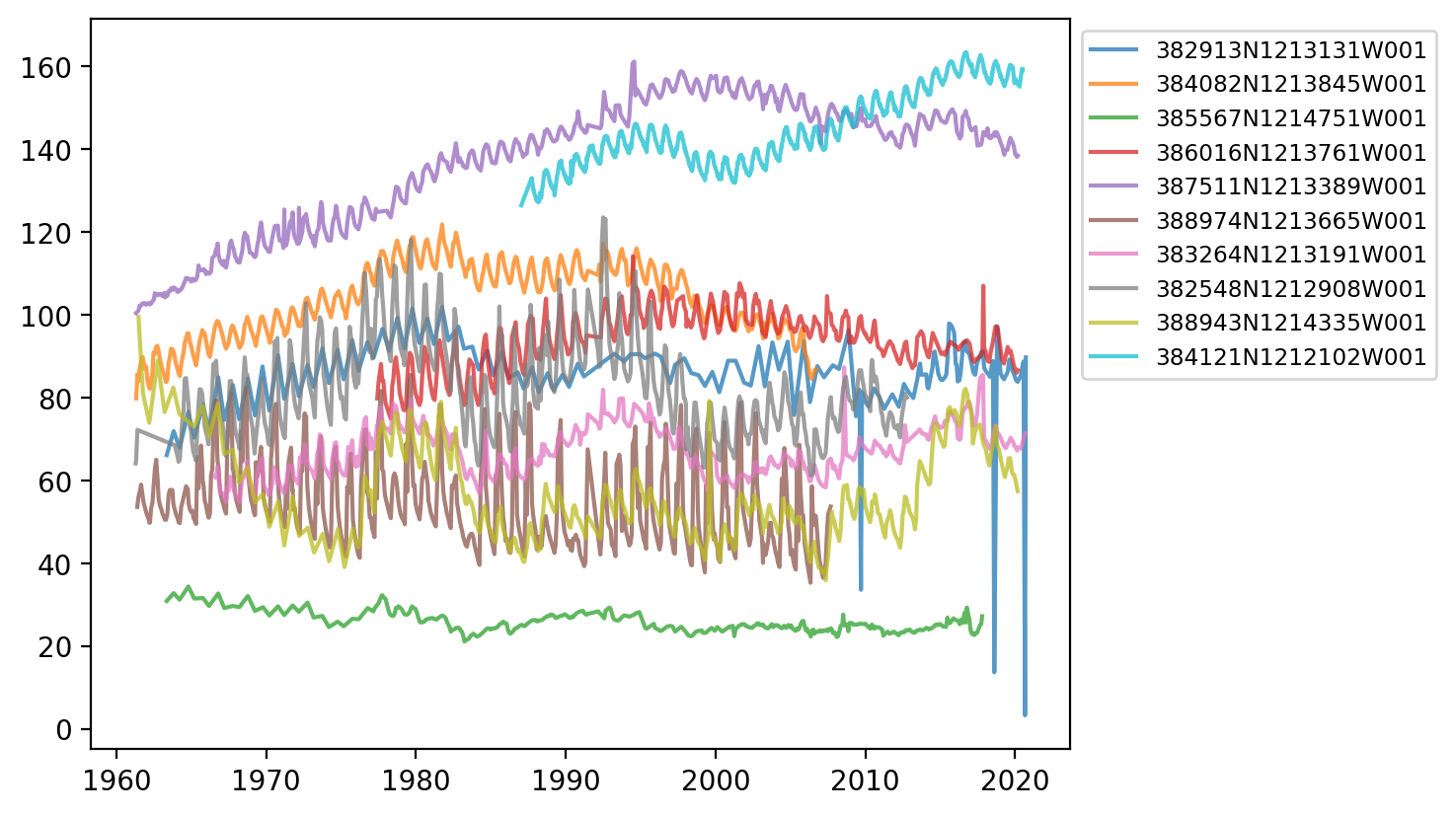
Going back to our original dataset of 10 different stations, lets plot all 10 in a loop onto the same Axes object. To tell the lines apart, we add a label= argument to each plot call, then add a legend box to the axis with the legend() method
fig, ax = plt.subplots(dpi=200)

for site_code in df_10.SITE_CODE.unique():
    df_site_code = df_10[df_10.SITE_CODE == site_code]
    ax.plot(df_site_code.MSMT_DATE, df_site_code.GSE_WSE, alpha=0.75, label=site_code)
ax.legend(
    fontsize="small",
    bbox_to_anchor=(1, 1),  # Shift legend outside of plot.
)
<matplotlib.legend.Legend at 0x15e0081a0>
Saving plots#
You can save a plot using the Figure’s savefig method. For instance, to save a pdf version of the most recent plot
fig.savefig("10-site-water-depth.pdf")
Even quicker in a noteook environment: right click on the plot, and copy/save as a PNG!
Plotting with seaborn#
With data that requires aggregation to plot (such as grouping or splitting), the seaborn package can handle much of the complexity for you.
Seaborn is normally imported with the sns abbreviation.
import seaborn as sns
Using seaborn with DataFrames is a little different than with matplotlib directly. You typically pass the whole DataFrame as a data argument, then the column names (rather than the data) as the x and y arguments.
Seaborn has it’s own scatter function (scatterplot):
fig, ax = plt.subplots(dpi=200)
sns.scatterplot(
    ax=ax,
    data=df_site,
    x="MSMT_DATE",
    y="GSE_WSE",
    alpha=0.5,
    color="black",
    s=6,
)
<Axes: xlabel='MSMT_DATE', ylabel='GSE_WSE'>
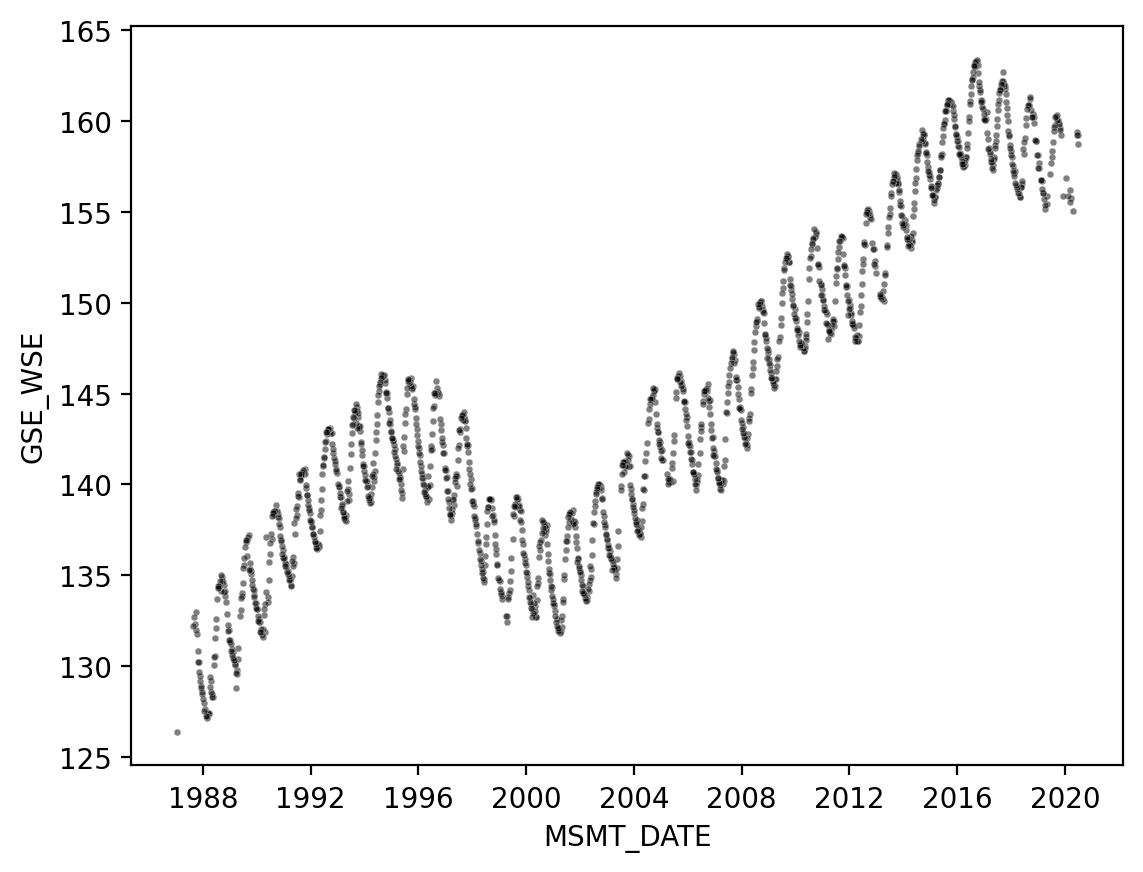
With seaborn, we still use a matplotlib Figure and Axes. But we automatically get axis labels!
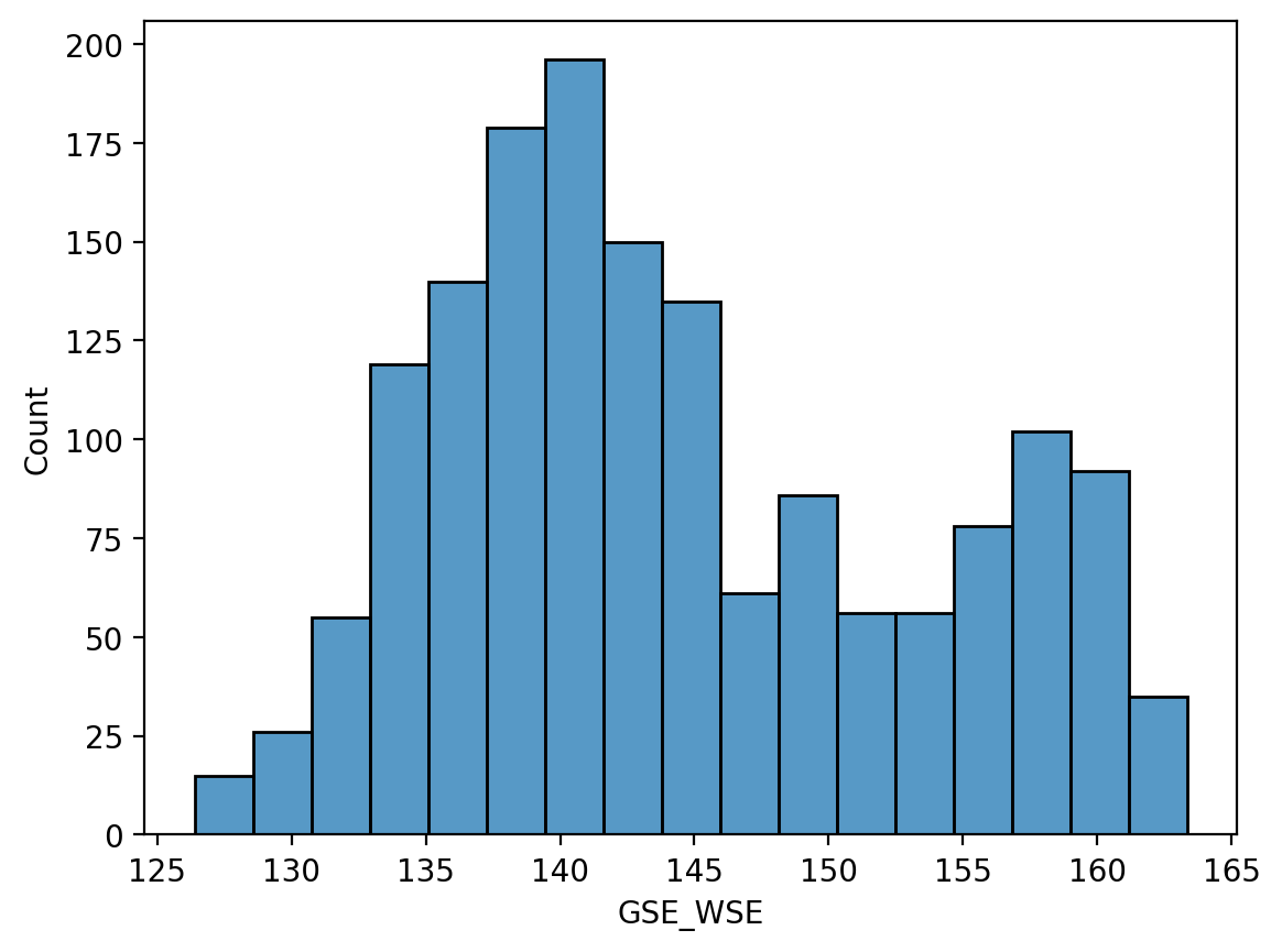
Most seaborn functions perform some data processing before plotting. For example, histplot calculates and plots a histogram
fig, ax = plt.subplots(dpi=200)
sns.histplot(ax=ax, data=df_site, x="GSE_WSE")
<Axes: xlabel='GSE_WSE', ylabel='Count'>
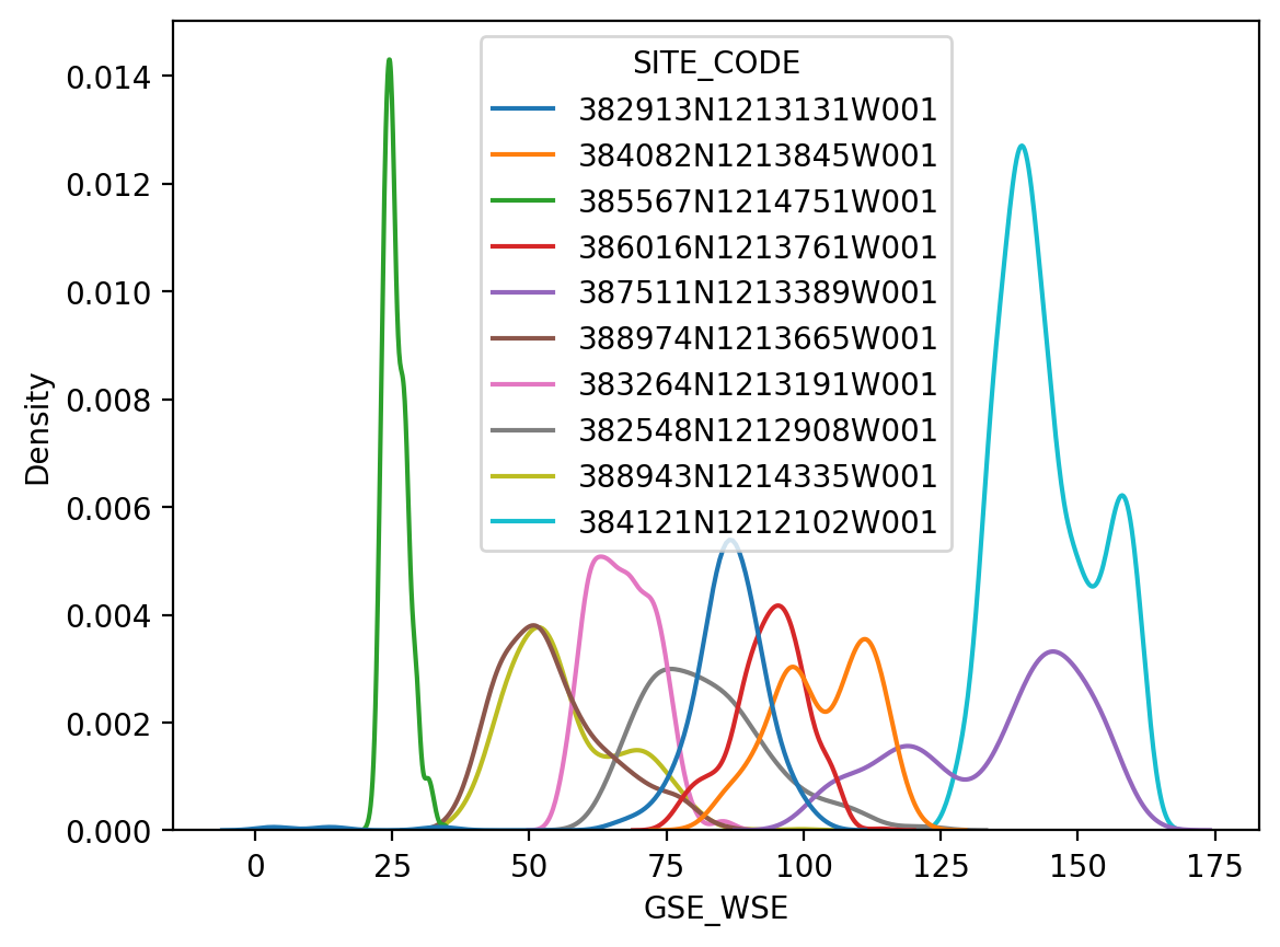
The thin lines of a KDE distribution plot (kdeplot()) make it easier to compare in the distribution of all 10 sites
fig, ax = plt.subplots(dpi=200)

sns.kdeplot(ax=ax, data=df_10, x="GSE_WSE", hue="SITE_CODE")
<Axes: xlabel='GSE_WSE', ylabel='Density'>
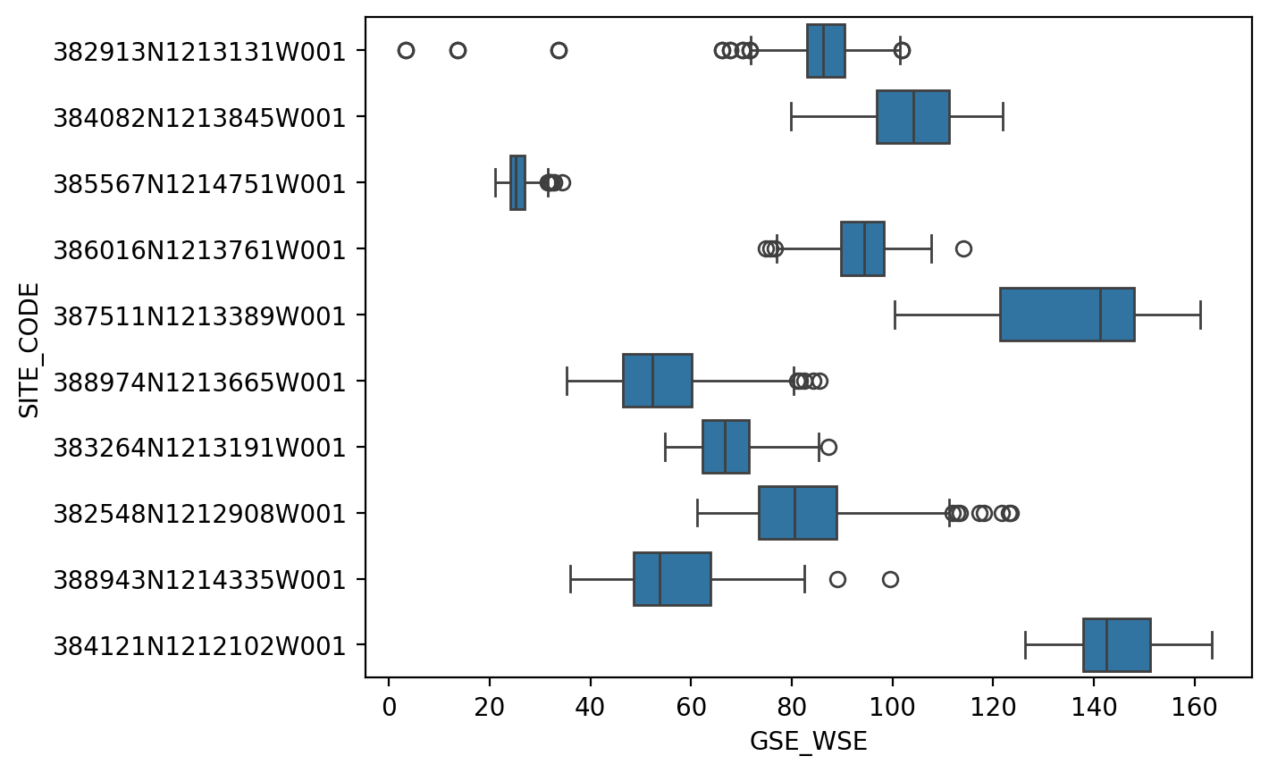
It’s still a little messy though, a box plot might be clearer still.
fig, ax = plt.subplots(dpi=200)
sns.boxplot(ax=ax, data=df_10, x="GSE_WSE", y="SITE_CODE")
<Axes: xlabel='GSE_WSE', ylabel='SITE_CODE'>
Seaborn has dozens of plot functions, mostly invoking comparing distributions of data.
The seaborn gallery is the place to go for a good overview of what seaborn can do.